What is nonlinear analysis in FEA? Why every structural engineer should master it

Linear analysis: a powerful simplification

To understand nonlinear analysis, it helps to start with what linear analysis assumes. A linear static analysis solves the equilibrium equation:

[K]{u} = {F}

where [K] is the stiffness matrix of the structure, {u} the vector of nodal displacements and {F} the vector of applied forces. The stiffness matrix is computed once, from the original geometry and the material properties, and it does not change during the solution. Three assumptions make this possible:

• Small displacements and rotations: the deformed shape is so close to the original shape that equilibrium can be written on the undeformed geometry.
• Linear elastic material: stress is proportional to strain, following Hooke's law, and the material returns to its original shape when the load is removed.
• Constant boundary conditions: the supports, the loads and the connections between parts do not change during loading. Contacts that are closed stay closed, gaps that are open stay open.

When these assumptions are satisfied, linear analysis has remarkable properties. The response is proportional to the load, so results can be scaled. Results of different load cases can be superposed. The solution is unique and is obtained in a single step. This is why linear analysis is fast, robust and widely used, and why most engineers start with it.

The danger is that the software does not check these assumptions for you. If you ask your model to behave linearly, it will, even when the real structure does not.

What is a nonlinear system?

Mathematically, a nonlinear system is one whose behavior is not equal to the sum of its parts. Its response does not satisfy the principle of superposition: the response to two loads applied together is not the sum of the responses to each load applied separately.

In structural terms, the response of the structure, meaning its displacements, internal loads and stresses, is no longer proportional to the applied loads. The reason is that the stiffness of the structure changes during loading. The stiffness depends on the geometry and on the material properties. In a linear analysis, both are assumed to be unchanged while the load is applied. In a nonlinear analysis, these changes are taken into account: the stiffness matrix becomes a function of the displacements, and it is updated as the structure deforms. The equilibrium equation becomes:

[K(u)]{u} = {P}

and, when the loads themselves depend on the deformation, as in contact problems:

[K(u)]{u} = {P(u)}

Because the stiffness depends on the unknown displacements, this equation can no longer be solved in one step. The load must be applied in increments, and iterations are needed at each increment to find the equilibrium. That is the essence of nonlinear finite element analysis.

The history of FEA reflects this difficulty. In the 1970s, most finite element programs had little or no nonlinear capability, and the first implementations required the analyst to intervene at every iteration. Today, nonlinear solvers use automated incremental and iterative algorithms with convergence criteria. They are far more powerful, but they still require the analyst to understand the deep interaction between the physics of the problem and its mathematical formulation. Nonlinear analysis can be an art, and without that understanding, it can also be a source of frustration.

The three types of nonlinearity

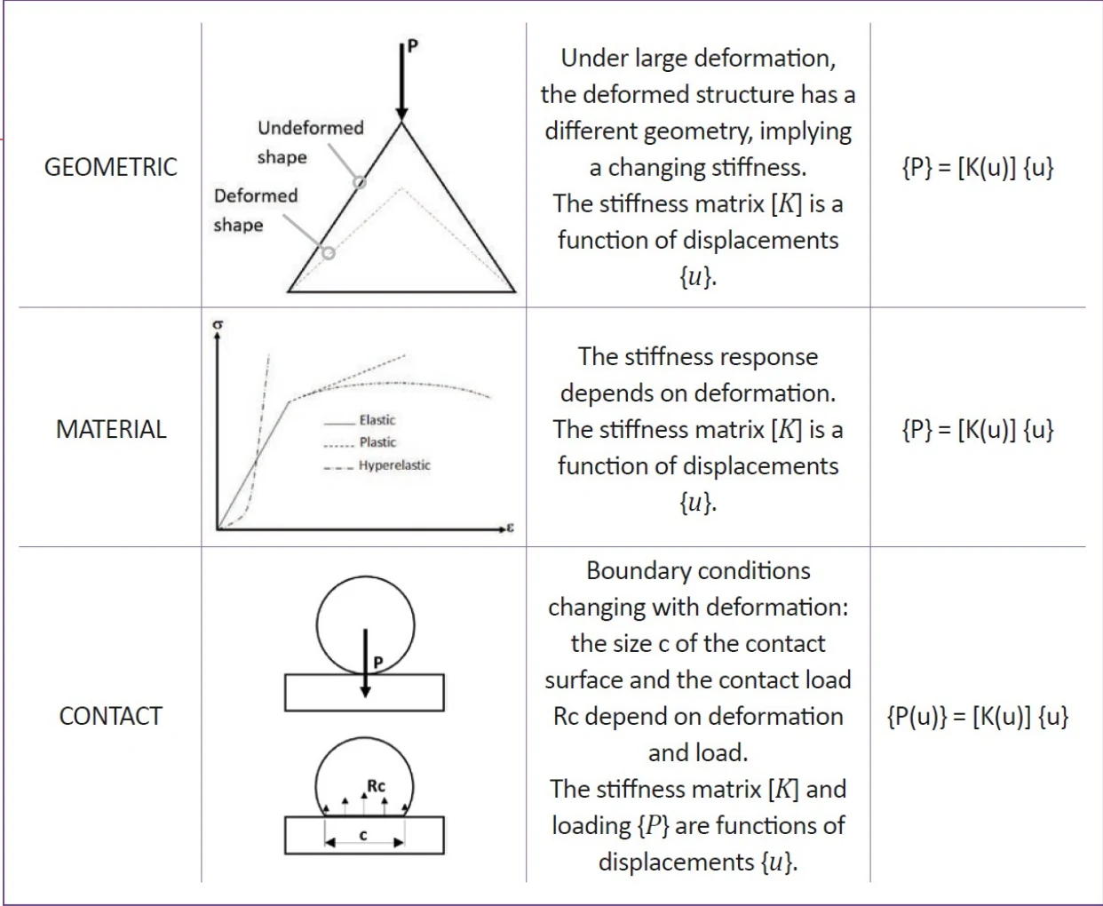
In structural analysis, a nonlinear behavior can come from three sources: the geometry, the material and the boundary conditions.

Geometric nonlinearity

Geometric nonlinearity appears when the deformation of the structure is large enough to change the way it carries the load. When a body undergoes large deformations, the strain-displacement relations become nonlinear, the deformed and undeformed shapes no longer coincide, and the stiffness changes with the deformation. New definitions of stress and strain are needed, and the geometry must be continuously updated.

There are three forms of geometric nonlinearity:

• Large deformations: when the shape of an element changes significantly, for example its cross section or thickness, its stiffness changes.
• Large rotations: when the orientation of an element changes significantly, its coordinates must be updated to compute equilibrium in the deformed configuration.
• Stress stiffening, or tension-bending coupling: the bending stiffness of an element increases because of the tension carried in its membrane. A plate under pressure is the classic example: as the plate deflects, membrane stresses develop, and they significantly increase its bending stiffness.

A simple example that shows everything

Consider a steel bar 2 m long and 1 cm in diameter, simply supported at both ends, with a person of 100 kg hanging from its middle. Intuition says that a steel bar can easily carry 100 kg over 2 m without dramatic deflection.

A linear analysis says otherwise. With a 1000 N load at mid-span, the maximum bending moment is 500 N·m, and the maximum bending stress computed by linear analysis is about 5,090 MPa, around thirteen times the ultimate strength of a basic structural steel. The linear analysis also predicts a mid-span deflection of 1.70 m, that is 85% of the length of the bar. According to the linear analysis, the bar cannot possibly carry the person.

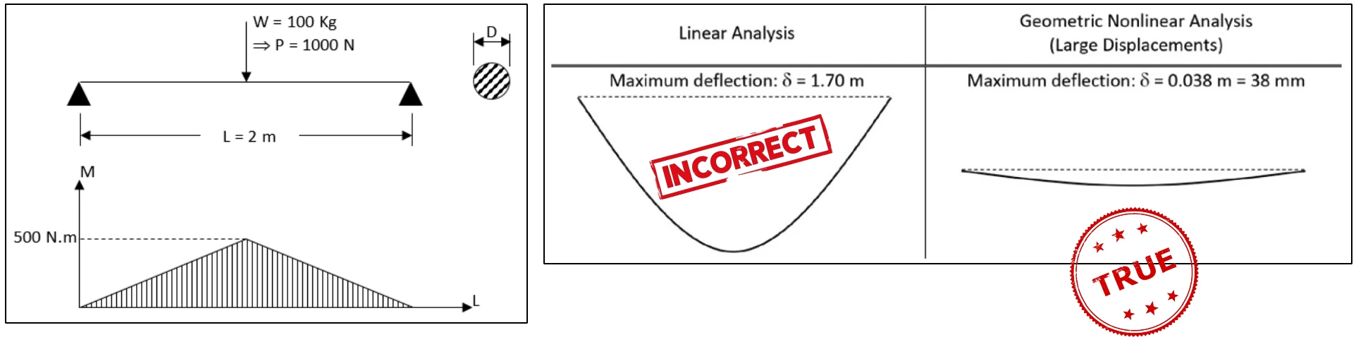
A geometric nonlinear analysis gives a completely different answer: a maximum deflection of about 38 mm. The reason is that, as the bar deflects, its supports prevent the ends from moving toward each other, so the bar stretches and develops a tensile force. In this example, the tension reaches about 11,900 N, while the bending moment at mid-span drops from 500 N·m to about 45 N·m. The bar carries the load mainly as a cable, through membrane tension, not as a beam in bending. This membrane effect can only be captured by a large displacement analysis.

The consequences go beyond the bar itself. If the bar is attached to two posts 5 m high, the tensile force in the bar pulls the tops of the posts inward and bends them. A linear analysis completely misses this horizontal force, so the posts would be designed without it and could be undersized.

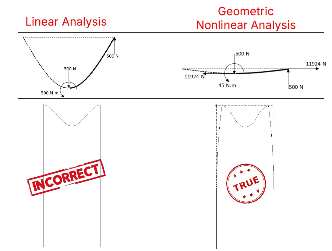
This simple example contains the main lessons of geometric nonlinearity: a linear analysis can be wrong by orders of magnitude, the error can be conservative in one place and unconservative in another, and the right answer requires the right assumption. If you tell your model to behave linearly, it will.

Follower loads

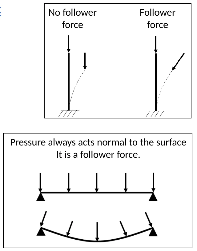
When the structure deforms significantly, a new question appears: does the load follow the deformation? The answer changes the results, and the software will not make the decision for you.

• Pressure is a follower load: it always acts normal to the surface, so its direction changes as the surface deforms.
• Gravity and inertia loads are not follower loads: they always act in the same direction.
• Enforced displacements and rotations are not follower loads: their direction is fixed by definition.
• Point forces have no general rule: it depends on the physical source of the force, and the analyst must use engineering judgment.
• Thermal loads are unaffected by the follower load choice.

Small strain or large strain?

Finally, geometric nonlinear problems can be small strain or large strain problems. In a small strain problem, the structure undergoes large displacements and rotations, but the elements themselves keep essentially the same shape. Most structural problems are of this type. In a large strain problem, the elements themselves deform significantly, as in metal forming or a rubber seal squeezed into its groove. Most FEA software uses the small strain formulation by default, so the analyst must explicitly activate the large strain option when it is needed, knowing that it requires more computing time.

Material nonlinearity

Material nonlinearity appears when the material no longer follows Hooke's law. For metallic structures, this means that the stress exceeds the proportional limit and the material starts to yield.

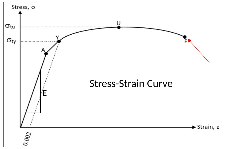
The stress-strain curve of a ductile metal, obtained from a tensile test, has four characteristic points:

• the proportional limit (point A), up to which stress is proportional to strain, with a slope equal to Young's modulus E;
• the yield point (point Y), usually defined by the 0.2% offset method, beyond which permanent plastic strain appears;
• the ultimate strength (point U), where necking begins;
• the fracture point (point F), where the specimen breaks.

Think of a paperclip. Bend it a little and it springs back: that is the elastic region. Bend it too far and it stays bent: the material has yielded and carries a permanent plastic strain. Beyond yield, most metals also strain harden: they become stronger as they deform plastically, which is why a paperclip is harder to bend back at the same spot.

To model this behavior, a nonlinear material model needs more than Young's modulus and Poisson's ratio:

• A stress-strain curve beyond yield, defined as a bilinear curve (yield stress and hardening slope), a multilinear curve from test data, or a mathematical model such as Ramberg-Osgood, widely used in aerospace for aluminum and titanium alloys.
• A yield criterion, which defines when a multiaxial stress state causes yielding. Von Mises is the usual choice for ductile metals; Tresca, Mohr-Coulomb and Drucker-Prager are used for other materials such as concrete and soils.
• A hardening rule, which defines how the yield surface evolves with plastic strain. Isotropic hardening expands the yield surface uniformly and is suitable for monotonic loading. Kinematic hardening translates the yield surface and captures the Bauschinger effect, essential for cyclic and reversed loading. Combined hardening uses both.
• The right stress and strain measures: engineering or true stress-strain data, consistent with the strain formulation used by the solver.

Why material nonlinearity matters

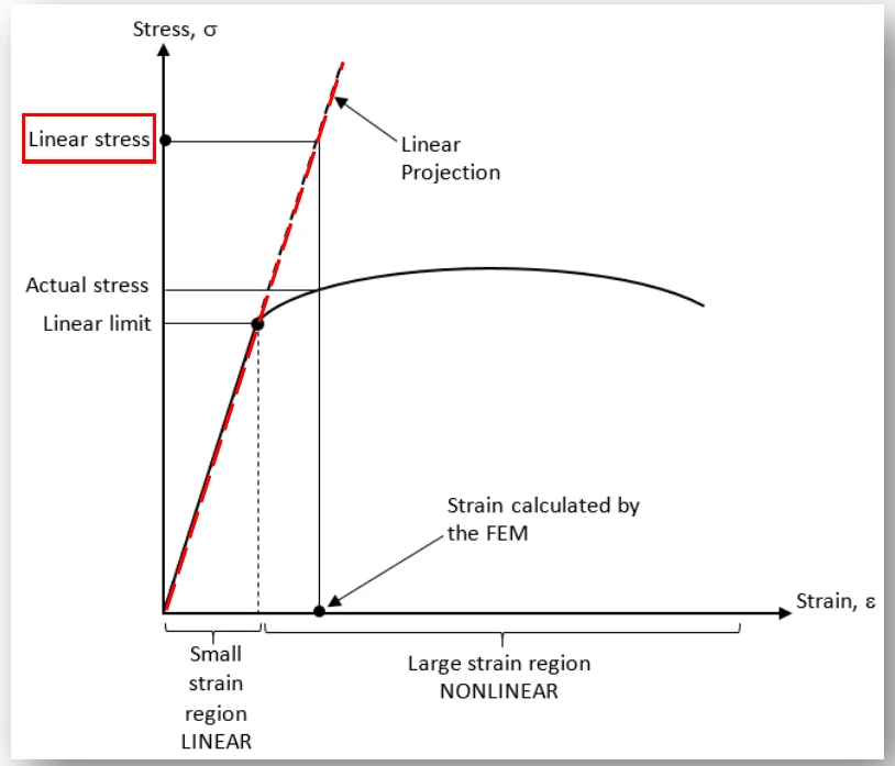
The first reason is accuracy. When a linear analysis is run on a part that yields, the solver continues to follow Hooke's law far beyond the proportional limit. The computed stress follows the linear projection of the elastic line, and the software reports a stress that can be much higher than the real one. The engineer may then conclude that the part fails when, in reality, it only yields locally and redistributes the load.

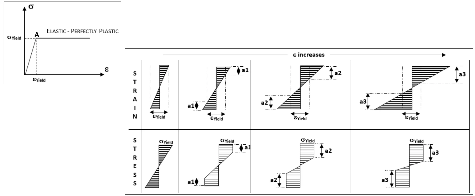
The second reason is capacity. Consider a beam in bending made of an elastic-perfectly plastic material. When the outer fibers reach yield, the beam is not yet at its limit: as the load increases, yielding spreads toward the neutral axis, and the inner fibers carry more of the load. Depending on the shape of the cross section, the additional bending capacity can reach 10% to 50% beyond first yield. A linear analysis cannot see this reserve. A nonlinear material analysis can, and it allows structures to be designed for their real capacity, with the right margins, instead of with unnecessary weight.

Yielding also allows load to be transferred from one part of a structure to another, which is essential to predict the behavior of joints, notches and redundant structures, and to evaluate residual stresses after an overload.

Boundary nonlinearity

Boundary nonlinearity appears when the boundary conditions change during loading. The most common case by far is contact: two surfaces that are separated may come into contact, surfaces in contact may separate, and surfaces in contact may slide relative to each other.

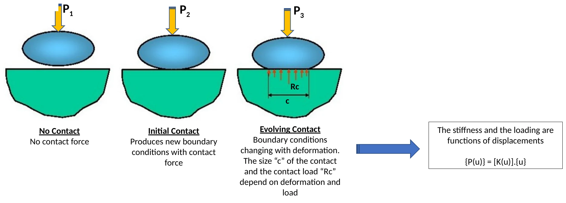
Consider a ball pressed onto a support. Before contact, there is no contact force. At first contact, new boundary conditions appear. As the load increases, the contact area grows and the contact force distribution changes. Both the stiffness and the loading become functions of the displacements. A linear analysis cannot handle this, because the status of the contact, open or closed, must be checked continuously during the solution.

Contact algorithms do exactly that. At each iteration, they measure the distance between the surfaces forming each contact pair. When a contact is detected as closed, forces are applied to prevent the surfaces from penetrating each other. When it is open, no load is transferred. Friction adds another layer: the tangential force depends on the normal force and on whether the surfaces stick or slip.

Contact is everywhere in real structures: bolted joints, where the load path through the clamped parts depends on which areas stay in contact; lugs and pins; bearings and gears; press fits; seals; parts resting on supports that can lift off. Other boundary nonlinearities include loads or constraints that change during the analysis, gaps that close, and cables that go slack.

In real structures, the three types of nonlinearity often appear together. The FEA Academy workshop below shows how to model a highly nonlinear problem that combines geometric nonlinearity, material nonlinearity and contact, step by step.

The eight characteristics of a nonlinear system

Whatever its source, a nonlinear system shares a set of characteristics that every analyst must keep in mind:

1. Load-displacement relation: the stiffness of the structure is not constant and varies with the applied loads. The displacements can become large and are no longer related to the original stiffness.
2. Stress-strain relation: stresses and strains are no longer related by a linear function.
3. Scalability: the results cannot be scaled. If you know the results for load P1, you cannot deduce the results for load P2; you must run both.
4. Superposition: the principle of superposition cannot be applied. Load cases cannot be combined by adding their results; each combination must be analyzed as a separate nonlinear case.
5. Initial state of stress: residual stresses, preloads and thermal states can strongly affect the response, and only a nonlinear solution can take them into account.
6. Load history: the response depends on the loading sequence. When several load steps are applied in sequence, the end state of one step is the initial state of the next.
7. Reversibility: the deformation is not necessarily reversible when the loads are removed. Plastic strains and residual stresses remain.
8. Solution settings: loads are applied in increments, iterations are needed to reach equilibrium, the solution must be monitored, computing times are longer, and the solution may fail to converge, or even converge to an incorrect answer.

How a nonlinear solver works

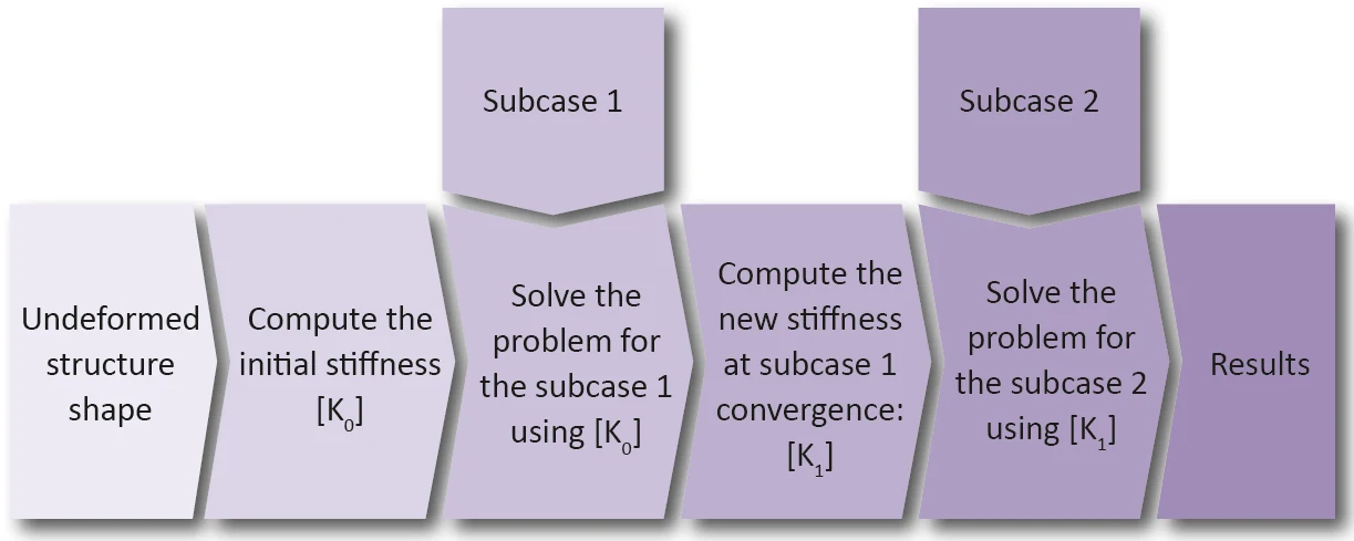
Because the stiffness depends on the displacements, a nonlinear solver cannot compute the answer in one step. It follows an incremental and iterative process.

The total load is divided into increments. For the first increment, the solver uses the initial stiffness to estimate the displacements. It then computes the internal forces corresponding to these displacements, using the updated geometry, material state and contact status, and compares them with the applied loads. The difference is the residual, the out-of-balance force. The solver then corrects the displacements and repeats the process, iterating until the residual is small enough according to the convergence criteria, typically based on forces, displacements or energy. Once the increment has converged, the next load increment is applied, starting from the converged state.

The most common iteration scheme is the Newton-Raphson method, which updates the stiffness matrix at every iteration and converges quickly near the solution. The modified Newton-Raphson method updates the stiffness less often, reducing the cost of each iteration at the price of more iterations. For problems where the load-displacement curve reaches a maximum and then decreases, such as buckling collapse or snap-through, load control fails at the peak; arc-length methods, such as the Riks method, control the progression along the equilibrium path instead and can follow the structure through its limit point.

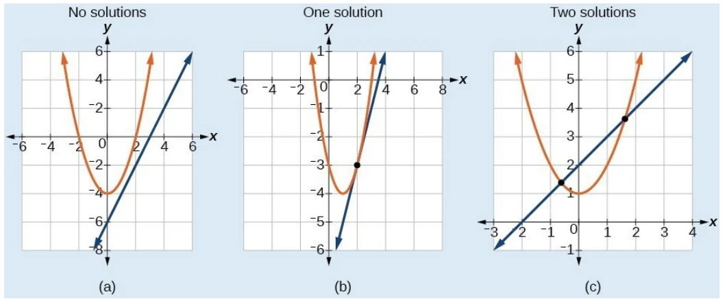
This process explains why nonlinear analysis requires more from the analyst than linear analysis. Linear problems always have a unique solution. Nonlinear problems may have no solution, one solution, or several, just as a nonlinear equation can have zero, one or two intersections with a straight line.

Load increments that are too large can make the solver miss the right equilibrium path. Convergence tolerances that are too loose can let it stop far from equilibrium. Artificial stabilization, offered by many codes to help difficult models converge, can add energy that changes the result. A nonlinear solution that "finished" is not necessarily a correct solution. Monitoring the convergence history, checking the energy balance and reading the solver messages are part of the analysis.

Do you really need a nonlinear analysis?

A nonlinear analysis requires more computing time, more disk space and more engineering time than a linear one. It is important to use it when it is needed, and only then. Two principles guide the decision:

• It is better to run a nonlinear analysis unnecessarily than to ignore a nonlinear effect when it is required. The first costs time; the second can lead to serious design errors.
• Nonlinear effects matter only when they are significant. A structure with small displacements, stresses below the proportional limit and no changing contacts is well served by a linear analysis.

The following guidelines help to decide.

For geometric nonlinearity:

• The 5% strain rule: if the maximum strain in the model exceeds 5%, a geometric nonlinear analysis is necessary.
• Look at the deformed shape at true scale: run the linear analysis and plot the deformed shape with a scale factor of 1.0. If it looks significantly different from the original shape, or different from what you expected, geometric nonlinearity is likely.
• Compare linear and nonlinear results on simple problems: if the displacements differ significantly, the nonlinear result must be used.
• Run a linear buckling analysis: low buckling eigenvalues reveal low bending stiffnesses and sensitivity to large deformations. Eigenvalues between 1.0 and 5.0 are a signal that nonlinear behavior should be considered, not only eigenvalues below 1.0.
• Watch slender members, which can buckle under compression or shear, and remember that bending can create compression.
• Watch thin-walled components: if a structure can develop a membrane state, it is a geometric nonlinear problem.

For material nonlinearity:

• If the stresses or strains do not exceed the proportional limit, there is no nonlinear material behavior. This requires knowing the yield limits of the materials.
• If a significant portion of the structure exceeds the proportional limit, a nonlinear material analysis is required.
• If the exceedance is limited to small regions, check whether it comes from a well-understood singularity far from the area of interest. If so, a linear analysis may remain acceptable.

For boundary nonlinearity:

• If parts can come into contact, separate or slide during loading, or if supports can lift off, the problem is nonlinear.
• If the load path through a joint depends on which surfaces are in contact, as in most bolted and pinned joints, contact must be modeled.

Where nonlinear analysis makes the difference

Nonlinear analysis is not an academic refinement. It is used every day to solve problems that linear analysis cannot handle:

• Aerospace thin-walled structures: fuselage and wing skin panels are often designed to buckle locally and continue to carry load in the post-buckling range. Predicting their real capacity requires geometric nonlinear analysis.
• Bolted and pinned joints: the distribution of loads between fasteners, the opening of joints under tension, and the stresses around holes depend on contact, preload and sometimes local yielding.
• Plates and membranes under pressure: tank walls, panels and diaphragms develop membrane stresses that a linear analysis ignores, leading to unrealistic bending stresses and deflections.
• Limit load and overload assessment: determining the real collapse load of a structure, or checking whether a structure survives an exceptional overload, requires plasticity and often large displacements.
• Seals, gaskets and elastomers: large strains, nonlinear materials and contact are all present at once.
• Forming and assembly processes: press fits, crimping, riveting and forming operations create residual stresses that change the behavior of the part in service.
• Failure investigations: understanding why a part failed usually means reproducing its behavior beyond the elastic range.
• Crash and impact: highly nonlinear and dynamic events, solved with explicit methods, are a field in themselves.

In many of these cases, a linear analysis would be either dangerously unconservative or so conservative that the design would be heavier and more expensive than necessary.

Why mastering nonlinear analysis matters for engineers

Modern FEA software has made nonlinear analysis easy to start. Activating large displacements, defining a plastic material or creating a contact pair takes a few clicks. That ease is precisely what makes mastering the subject so important.

Because the errors are bigger. In linear analysis, a modeling error usually produces a result that is wrong by some percentage. In nonlinear analysis, the wrong assumption can change the answer by an order of magnitude, as the simple bar example shows, or produce a converged solution on the wrong equilibrium path.

Because the software will not decide for you. Whether a load follows the deformation, which hardening rule fits the loading, whether strains are small or large, how to define contact, how large the load increments should be: these are engineering decisions. The defaults are designed to run, not to be right for your problem.

Because it leads to better designs. Nonlinear analysis reveals the real capacity of a structure: the reserve after first yield, the strength of a panel after buckling, the real load path through a joint. Engineers who master it can design lighter, more efficient structures with justified margins, instead of compensating for uncertainty with extra material.

Because demanding projects require it. Aerospace certification, nuclear and pressure equipment codes, offshore structures and safety-critical products routinely require nonlinear analyses. Engineers who can plan, run, check and defend these analyses are trusted with the most challenging work.

Because it builds engineering judgment. Understanding why a structure behaves nonlinearly deepens your understanding of structural behavior in general. It makes you a better linear analyst too, because you know exactly when the linear assumptions hold and when they do not.

In short, nonlinear analysis is where finite element analysis stops being a tool that anyone can operate and becomes a discipline that rewards knowledge, method and experience.

Common pitfalls in nonlinear analysis

Experience shows that the same mistakes come back again and again:

• running a linear analysis on a structure that clearly yields or deforms significantly, and reporting the resulting stresses;
• using engineering stress-strain data where true stress-strain data is required, or the reverse;
• choosing isotropic hardening for a structure under reversed or cyclic loading;
• forgetting to decide whether pressure and point loads are follower loads;
• using load increments that are too large, or convergence tolerances that are too loose;
• relying on artificial stabilization without checking how much energy it adds;
• combining nonlinear load cases by superposition;
• accepting a "converged" solution without checking the deformed shape, the reaction forces and the energy balance;
• modeling contact with a mesh that is too coarse to represent the contact pressure distribution.

Each of these mistakes can produce a result that looks perfectly plausible. Avoiding them requires understanding, not just software skills.

How to learn nonlinear FEA

Nonlinear analysis builds on the fundamentals of linear FEA: elements, meshing, boundary conditions, loads and verification. Engineers who have a solid foundation in these topics are ready to learn the three types of nonlinearity, the solution strategies, and the modeling techniques that make nonlinear analyses reliable.

The on-demand course Practical Nonlinear FEA covers these topics in depth, from geometric, material and boundary nonlinearity to solution strategies, convergence, contact modeling and nonlinear buckling, with 15 lectures and 17 workflow videos. It is software-agnostic: the principles apply to any FEA package. The book Practical Finite Element Analysis for Mechanical Engineers also dedicates a chapter to nonlinear analysis, with practical guidelines and examples.

Conclusion

Nonlinear analysis is what allows a finite element model to follow a structure when it deforms significantly, when its material yields, or when its contacts open, close and slide. It is required whenever the stiffness of the structure changes during loading, which happens far more often in real engineering than in textbook examples.

A linear analysis remains the right starting point for many problems, and a good engineer knows when it is sufficient. But a good engineer also knows when it is not: when a membrane carries the load, when a section yields, when a joint opens, when a panel buckles. In those situations, a linear analysis can be wrong by orders of magnitude, on the safe or on the unsafe side.

Mastering nonlinear analysis means understanding the physics behind each type of nonlinearity, making the right modeling decisions, guiding the solver to a converged and correct solution, and checking the result with engineering judgment. It is one of the most demanding skills in finite element analysis, and one of the most rewarding: it gives engineers the ability to predict how real structures behave, and to design them with confidence.

See all articles