
"How accurate is FEA?" is one of the most common questions engineers ask, and one of the most difficult to answer in a single sentence. A finite element model can predict the stiffness of a bracket within one or two percent of a strain-gauge test. The same software, in other hands, can predict a stress that is off by a factor of three, with a colorful contour plot that looks perfectly convincing. The method is the same in both cases. What changes is everything the engineer puts into the model and everything the engineer does to check what comes out of it.
The short answer is that FEA is as accurate as the model is good. The accuracy of a finite element analysis is not a property of the software. It is a property of the complete chain of decisions that goes from the physical problem to the numbers in the report: the mesh, the material data, the boundary conditions, the assumptions, the solver settings, the level of complexity, the convergence checks, the validation, and the expertise of the person who connects all of these. This article walks through each of these factors, explains how each one can make your results more or less accurate, and gives practical ways to keep the error under control.
What "accuracy" means in FEA
Before looking at the factors, it helps to be precise about what we mean by accuracy. When an FEA result differs from what happens in reality, the difference comes from three distinct sources, and each one requires a different response.
- Modeling error: the mathematical model you chose does not represent the physical reality. You assumed linear material behavior when the part yields, you fixed a boundary that moves in reality, or you ignored a contact that opens under load. No amount of mesh refinement removes this error, because the equations themselves are not the right ones.
- Discretization error: the finite element solution is an approximation of the exact solution of the mathematical model. The elements can only represent a limited set of displacement shapes, so a coarse mesh gives an approximate answer. This error decreases as the mesh is refined, and it can be estimated.
- Numerical error: round-off, ill-conditioning of the stiffness matrix, and convergence tolerances in iterative or nonlinear solutions. With modern solvers and double precision, this error is usually small, but it becomes significant with badly scaled models, very stiff connections next to very flexible parts, or loose convergence criteria.
This decomposition is the basis of the two activities that every serious FEA process includes. Verification answers the question "Am I solving the equations right?" and addresses discretization and numerical errors. Validation answers the question "Am I solving the right equations?" and addresses modeling error by comparing predictions with physical reality. A model can be perfectly verified and still be wrong, because it solves the wrong problem with great precision.
It also helps to remember that accuracy depends on the quantity you look at. Displacements are the primary unknowns of a displacement-based finite element model and they converge fastest. Stresses are derived from the derivatives of the displacements, so they converge more slowly and are more sensitive to the mesh. Peak stresses at notches, holes and fillets are the most sensitive of all. A model can predict the global stiffness of an assembly within a few percent and still underestimate a local peak stress by thirty percent. When someone asks "how accurate is my model?", the first answer should be another question: "accurate for which result?"
1. Mesh quality
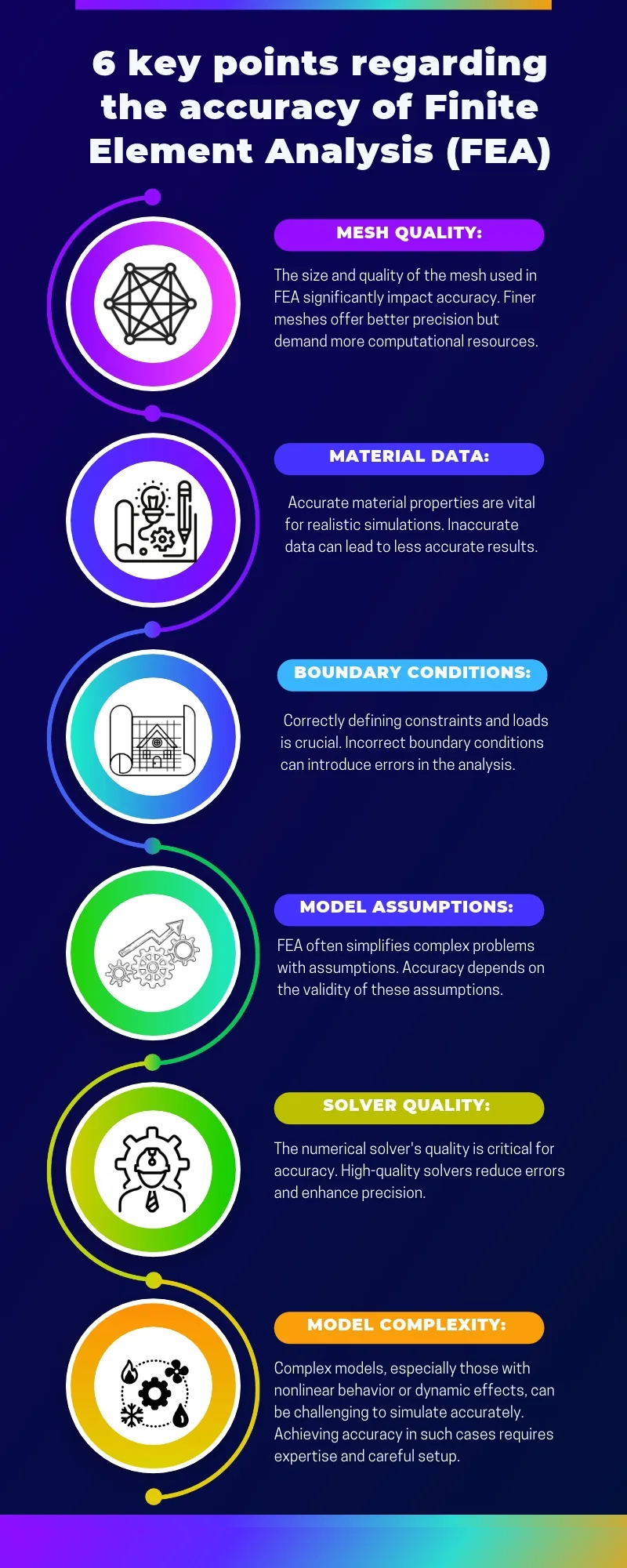
The mesh is the most visible part of a finite element model, and its quality has a direct effect on accuracy. The size and the quality of the elements control how well the model can represent the real distribution of displacements and stresses. Finer meshes give better precision, but they demand more computational resources, so the engineer always looks for the right balance.
Element size and convergence
Each element can only represent a limited set of displacement shapes. A linear tetrahedral element, for example, can only represent a constant strain inside its volume. Where the stress changes rapidly, around a hole or a fillet radius, a coarse mesh of such elements cannot follow the gradient, and the peak stress is underestimated. As the elements become smaller, the solution approaches the exact solution of the mathematical model. This is the principle of mesh convergence.
The practical consequence is simple: a single mesh tells you nothing about its own accuracy. To know whether your mesh is good enough, you need to compare at least two, and preferably three, meshes of increasing density in the area of interest. If the result of interest changes by less than a few percent between the last two meshes, the mesh is converged for that result. If it keeps changing, you need to refine further, or you may be looking at a singularity.
Singularities
A sharp re-entrant corner, a point load, or a point constraint creates a stress singularity: the theoretical stress at that point is infinite. In the finite element model, the stress at a singularity never converges. It keeps increasing every time you refine the mesh. Engineers who do not recognize singularities either report meaningless peak values or conclude that the model "does not converge". The right response is to recognize the singularity, to model the real geometry (a fillet radius instead of a sharp corner, a distributed load instead of a point load), or to evaluate the stress at a distance from the singular point where the result is meaningful.
Element shape and type
Accuracy also depends on the shape of the elements. Elements with high aspect ratios, strong warping, large skew angles or poor Jacobians degrade the solution, especially for stresses. Most preprocessors provide quality checks for these criteria, and they should be run on every model before solving.
The element type matters just as much as the element shape. First-order tetrahedral elements are notoriously stiff in bending and should be avoided for stress analysis unless the mesh is very fine. Second-order tetrahedral elements perform much better. Thin-walled structures are usually better represented by shell elements than by several layers of solid elements, and slender members by beam elements. Choosing the element type is a modeling decision that affects accuracy before the first element is even created.
Practical guidelines
- Refine the mesh where the stress gradients are high, and keep it coarser where the stress field is uniform.
- Perform a mesh convergence study on the results that matter for your decision.
- Check element quality criteria before solving.
- Learn to recognize singularities and treat them correctly instead of chasing them with ever finer meshes.
2. Material data
The finite element model can only be as accurate as the material data it uses. Accurate material properties are vital for realistic simulations, and inaccurate data leads to inaccurate results, whatever the quality of the mesh.
For a linear static analysis of an isotropic metal, the material model needs only two elastic constants, Young's modulus and Poisson's ratio, plus the density if gravity or inertia loads are applied. These values are well known for common alloys, and the error they introduce is usually small. The situation changes quickly as the problem becomes more complex:
- Composite materials require orthotropic or anisotropic properties, ply orientations, stacking sequences and allowables that depend on the manufacturing process. Small errors in ply angles or in the transverse properties can change the stiffness and the failure predictions significantly.
- Nonlinear materials require stress-strain curves, hardening laws and sometimes rate dependency. The difference between engineering and true stress-strain data, or the extrapolation of a curve beyond the tested range, can change the predicted plastic strain by a large amount.
- Polymers and elastomers are sensitive to temperature, strain rate and time. A hyperelastic model fitted to a uniaxial test only can behave poorly in shear or biaxial loading.
- Temperature-dependent properties are needed whenever the structure operates over a wide temperature range.
Material data also carries scatter. Two batches of the same alloy do not have exactly the same properties, and design allowables are statistical values chosen to cover this scatter. When the analysis is used to justify a design, the engineer must know whether the properties used are typical values or design allowables, and use them consistently with the applicable standard.
The practical rule is to know where your material data comes from. Use data from reliable sources such as recognized handbooks, supplier certificates or your own test program, document it, and make sure it covers the conditions of your analysis: temperature, strain range, loading rate and environment.
3. Boundary conditions
Boundary conditions define how the model is supported and how it is loaded. Correctly defining constraints and loads is crucial: incorrect boundary conditions introduce errors in the analysis that are often much larger than the discretization error, and they are among the most frequent sources of wrong FEA results.
The difficulty is that real structures are rarely supported by the idealized constraints available in FEA software. A bolted flange is not fully fixed, and it is not free either. A shaft in a bearing can rotate, but only within the clearance of the bearing. A part that sits on another part can lift off. When the engineer fixes every node on a face because it is "attached" to something, the model becomes artificially stiff, the displacements are underestimated, and the stresses near the constraint can be completely wrong.
Some common problems:
- Over-constraining: fixing all degrees of freedom where the real structure can deform or slide. The model is too stiff, and spurious stresses appear at the constraint.
- Under-constraining: leaving rigid body motions free in a static analysis. The solver fails or returns meaningless displacements.
- Unrealistic load introduction: applying a load at a single node or on a small face creates a local stress concentration that does not exist in reality.
- Wrong load path: forgetting a load case, applying a load in the wrong coordinate system, or using the wrong units.
Saint-Venant's principle helps here: the details of how a load or a constraint is applied affect the stresses only in a region close to where it is applied. This means you can often idealize supports and loads far from the area of interest, provided you do not use the stresses in that region. It also means that the area of interest must be far enough from the idealized boundaries, or the boundaries must be modeled realistically, for example by including part of the surrounding structure.
A useful habit is to check the reaction forces after every run. The sum of the reactions must balance the applied loads, and their distribution must make engineering sense. If 90 percent of the load goes through a support that should carry half of it, the boundary conditions are wrong, whatever the quality of the mesh.
4. Model assumptions
Every finite element model is a simplification of a complex reality. FEA always relies on assumptions, and the accuracy of the results depends on the validity of these assumptions. This is the source of the modeling error described at the beginning of this article, and it is the one that refinement cannot fix.
Typical assumptions include:
- Geometric simplifications: removing small holes, fillets, chamfers and fasteners that are not important for the result of interest. This is often necessary and sensible, but a removed fillet can be exactly where the part will crack.
- Linear behavior: assuming small displacements, linear elastic material and fixed contact conditions. Linear analysis is fast and robust, but it gives wrong answers when displacements are large, when the material yields, or when contacts open and close.
- Idealized connections: representing bolts, welds, rivets and adhesive joints with rigid elements, springs or tied contacts. The stiffness of these connections controls the load distribution in an assembly.
- Symmetry: using a half or a quarter model is efficient, but only when the geometry, the material, the loads and the boundary conditions are all symmetric. Symmetric models also hide antisymmetric buckling and vibration modes.
- Static versus dynamic: treating a load as static when its frequency content is close to a natural frequency of the structure.
The right attitude toward assumptions is to make them explicitly, to write them down, and to check them. If you assume linear behavior, check that the stresses stay below the yield strength and that the displacements are small compared with the dimensions of the structure. If you assume a connection is rigid, check how sensitive the result is to its stiffness. An assumption that is documented and checked is engineering. An assumption that is made by default, because it is the default in the software, is a risk.
5. Solver quality and solver settings
The numerical solver turns the finite element model into numbers. The quality of the solver is critical for accuracy, and modern commercial and open-source solvers are mature, well-tested codes that reduce numerical errors to a minimum for most applications.
In practice, the engineer has more influence on the solver accuracy through the choice of the solution type and the settings than through the choice of the code itself:
- Analysis type: a linear static solution cannot capture buckling, plasticity or contact. A linear buckling solution gives an eigenvalue, not a collapse load. A modal analysis gives natural frequencies and mode shapes, not response amplitudes. Choosing the solution that matches the physics is the first condition of accuracy.
- Direct versus iterative solvers: direct solvers are robust and accurate, iterative solvers are faster for large models but depend on convergence tolerances and preconditioning.
- Nonlinear settings: load increments, convergence criteria for force, displacement and energy, line searches, and stabilization. Loose tolerances give fast but inaccurate solutions. Artificial stabilization can make a model converge while adding energy that changes the result.
- Dynamic settings: time step size, damping, and the number of modes retained in a modal superposition analysis.
- Numerical conditioning: very large differences in stiffness between connected parts, or rigid elements connected to very flexible regions, degrade the conditioning of the stiffness matrix. Solvers usually report this with warnings about singularities or high ratios. These warnings must be read and understood, not ignored.
The solver output file is part of the result. It contains warnings, error messages, energy balances, and convergence histories. Reading it is one of the simplest and most neglected ways of catching an inaccurate solution before it reaches a report.
6. Model complexity
Complex models, especially those with nonlinear behavior or dynamic effects, are challenging to simulate accurately. Achieving accuracy in such cases requires expertise and careful setup.
Complexity has two faces. On one side, a more complex model can capture more of the physics: contacts, plasticity, large displacements, temperature fields, fluid interaction. On the other side, every additional feature adds parameters that must be defined correctly, increases the solution time, and creates new ways for the model to fail or to give misleading results. A large assembly with hundreds of contact pairs can take days to converge, and when it finally does, verifying that every contact behaves correctly is a project in itself.
The guiding principle is to build the simplest model that answers the question. Start with a simple model, understand its results, and add complexity only where it changes the answer. A linear model run first gives a reference: if the stresses are far below yield, a nonlinear material model may not be needed. A coarse global model run first shows the load paths and tells you where a detailed submodel is needed. This progressive approach is faster, and it gives the engineer an understanding of the structure that a single complex model never provides.
Beyond the six factors: convergence, validation and expertise
The six key points above cover what goes into the model. Three more factors determine whether the results that come out of it can be trusted.
Convergence
Convergence has two meanings in FEA, and both matter. Mesh convergence, discussed above, checks that the discretization error is small for the result of interest. Solution convergence, in nonlinear analysis, checks that the iterative solution has found equilibrium at each load increment within acceptable tolerances. A nonlinear solution that "finishes" with loose tolerances, or that needs a large amount of artificial stabilization to finish, may not be in equilibrium at all. Checking the convergence history and the energy balance is part of the analysis, not an optional extra.
Validation
When it is necessary, and particularly when the analysis supports a critical decision, FEA results should be validated against physical tests or benchmarks. Validation can take several forms:
- comparison with analytical solutions for simple configurations, such as beam theory, plate theory or classical stress concentration factors;
- comparison with benchmark problems, such as those published by NAFEMS, which provide reference solutions for standard problems;
- comparison with physical tests, from coupon tests to component and full-scale tests, using strain gauges, displacement measurements or digital image correlation;
- comparison with service experience on similar structures.
Validation is what turns a model into a predictive tool. A model that has been correlated with a test on one configuration can then be used with confidence to explore variations of that configuration, which is where simulation brings its full value.
Expertise
The last factor is the one that connects all the others: the expertise of the engineer. Software has become easy to use, and that is a good thing, but it also means that a model can be built and solved without understanding what the elements do, what the boundary conditions imply, or what the solver warnings mean. The accuracy of an FEA does not come from the software; it comes from the engineering judgment applied at every step.
Expertise shows in simple habits: estimating the expected result with a hand calculation before running the model, checking the deformed shape for plausibility, checking the reaction forces, questioning a result that seems too good or too bad, and knowing the limits of each modeling choice. These habits catch most errors long before a test does.
A practical checklist for accurate FEA
To ensure accurate results, it is essential to consider these factors carefully and, when necessary, to validate FEA outcomes against physical tests or benchmarks. The following checklist summarizes the article:
| Factor | Question to ask | Typical check |
|---|---|---|
| Mesh quality | Is the mesh fine enough where the results matter? | Mesh convergence study, element quality checks |
| Material data | Where do the properties come from, and do they cover the conditions of the analysis? | Documented sources, temperature and strain range |
| Boundary conditions | Do the supports and loads represent the real structure? | Reaction forces, load balance, deformed shape |
| Model assumptions | Which assumptions did I make, and are they valid? | Written list of assumptions, sensitivity checks |
| Solver | Is the solution type right, and are the settings appropriate? | Output file warnings, convergence history, energy balance |
| Model complexity | Is this the simplest model that answers the question? | Progressive approach, comparison with a simpler model |
| Convergence | Is the solution converged, both in mesh and in iterations? | Two or three meshes, nonlinear convergence criteria |
| Validation | Has the model been compared with reality? | Hand calculations, benchmarks, test correlation |
Conclusion
So, how accurate is FEA? When the model is built with the right elements and a converged mesh, reliable material data, realistic boundary conditions, documented and checked assumptions, an appropriate solver, and a level of complexity that matches the question, finite element analysis is remarkably accurate. It routinely predicts stiffness, natural frequencies and stresses within a few percent of test results, and it is used every day to certify aircraft, cars and medical devices.
When any link of that chain is weak, FEA becomes a machine for producing precise-looking wrong answers. The difference between the two outcomes is not the software. It is the method and the judgment of the engineer. That is why learning FEA is not about learning which buttons to click, but about learning how to make, check and document each of the decisions described in this article.

Go further
Learn FEA with a structured path: the on-demand course Practical Basic FEA covers the fundamentals step by step, and Practical Finite Element Analysis for Mechanical Engineers by Dominique Madier gathers the best modeling practices in one book.
See the Practical Basic FEA course Take the free FEA diagnostic