The FEA process: thirteen steps from problem definition to engineering decision

Why a structured process matters

An FEA model can be built in a few hours with modern software. It can also be wrong in a few hours. Most errors found in finite element analyses are not software bugs. They are process errors: an analysis that answers the wrong question, a boundary condition that does not represent the real support, a material curve taken from the wrong temperature, a result reported without a convergence check, or a conclusion that nobody can reproduce because the assumptions were never written down.

A structured process protects against these errors in three ways. It forces the engineer to make decisions explicitly instead of accepting software defaults. It creates natural checkpoints where errors can be caught before they propagate. And it produces a trail of documentation that allows a colleague, a manager or a certification authority to understand and trust the result. In many organizations, this process is formalized as a Standard Operating Procedure (SOP) for FEA.

The thirteen steps can be grouped into four phases:

1. Preparing the analysis: problem definition, geometry preparation, mesh generation, material properties and boundary conditions (steps 1 to 5).
2. Solving and interpreting: solver setup, analysis and post-processing (steps 6 to 8).
3. Checking and improving: validation and optimization (steps 9 and 10).
4. Delivering: documentation, decision-making and iteration (steps 11 to 13).

Phase 1: preparing the analysis

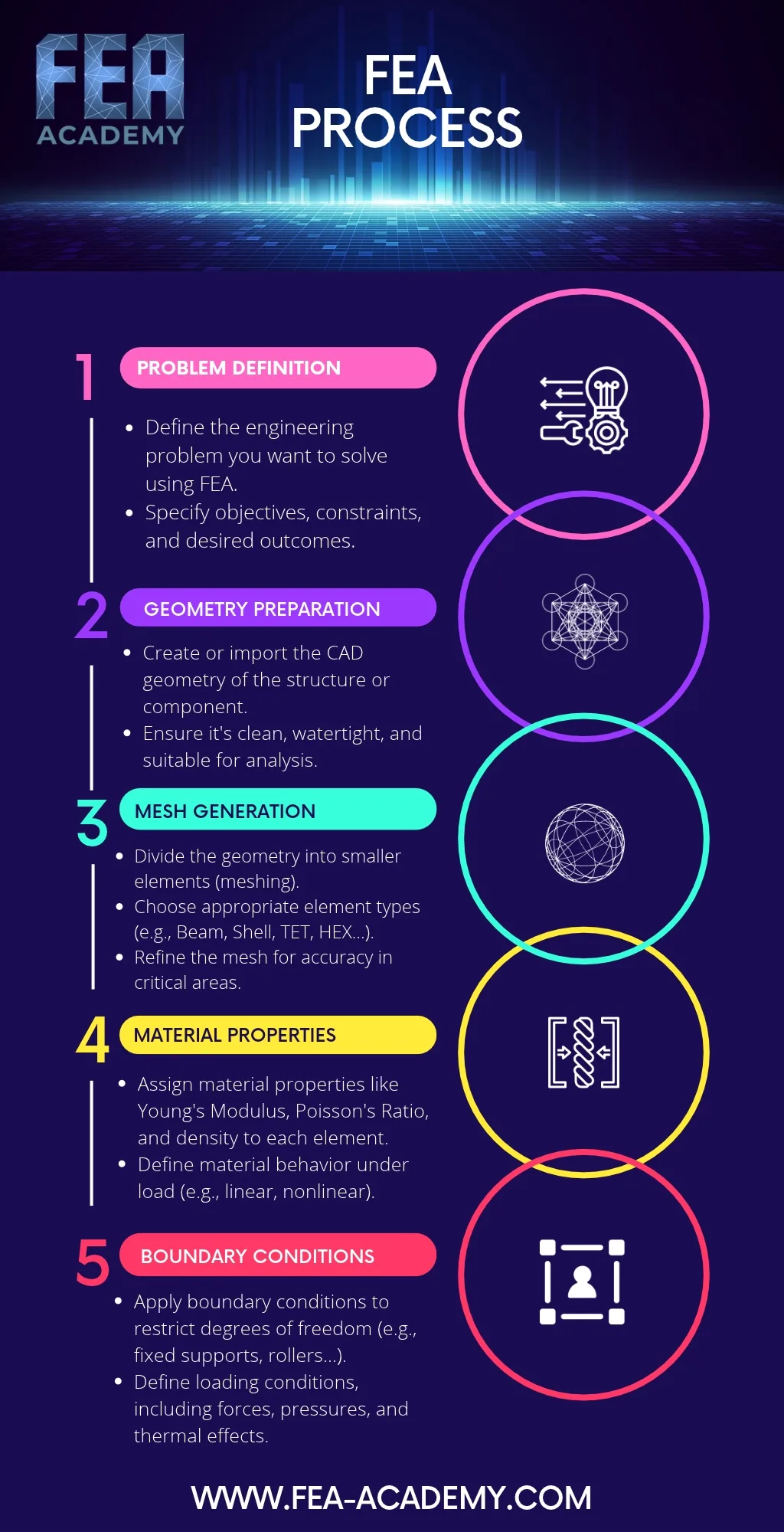
Step 1: Problem definition

Define the engineering problem you want to solve using FEA. Specify the objectives, the constraints and the desired outcomes.

This is the most important step of the process, and the one most often skipped. "Run an FEA on this part" is not a problem definition. A problem definition answers questions such as:

• What decision will this analysis support? Sizing a part, approving a design change, investigating a failure, comparing two concepts?
• Which results are needed? Maximum stress, margin of safety, displacement at a specific point, natural frequencies, buckling load, fatigue life?
• Which load cases and environments must be considered?
• What accuracy is needed, and what are the acceptance criteria?
• What are the constraints in time, budget and computing resources?

The answers to these questions determine every later step: the level of geometric detail, the element types, the mesh density, the analysis type and the format of the report. An analysis without a clear problem definition tends to grow without limit, because there is no criterion for deciding when it is good enough.

A good practice is to write the problem definition down in a few lines and to agree on it with the person who will use the results. It is also the right moment to make a first estimate of the expected result with a hand calculation. This estimate will be invaluable later to check the FEA results.

Step 2: Geometry preparation

Create or import the CAD geometry of the structure or component. Ensure it is clean, watertight and suitable for analysis.

The CAD model is designed for manufacturing, not for analysis. It contains details that are essential for production but irrelevant or harmful for the analysis: small fillets, chamfers, logos, threads, tiny holes. It may also contain defects, such as small gaps between surfaces, overlapping faces or sliver surfaces, that prevent a good mesh.

Geometry preparation, sometimes called defeaturing or idealization, transforms the CAD model into an analysis model:

• Cleaning: repairing gaps, removing duplicate surfaces, closing volumes so that they are watertight.
• Defeaturing: removing details that do not influence the results of interest. The key word is "of interest": a small fillet can be removed from a region of low stress, but it must be kept where the stress is evaluated.
• Idealization: extracting mid-surfaces for shell elements in thin-walled parts, or lines for beam elements in slender members.
• Partitioning: splitting the geometry to control the mesh, to apply loads on specific areas, or to prepare regions with different mesh densities.

The result should be the simplest geometry that still represents the structural behavior needed to answer the question defined in step 1.

Step 3: Mesh generation

Divide the geometry into smaller elements. Choose appropriate element types (beam, shell, tetrahedral, hexahedral). Refine the mesh for accuracy in critical areas.

Meshing is where the continuous structure becomes a finite element model. Two decisions dominate this step.

The first is the choice of element type. Beam elements represent slender members efficiently. Shell elements represent thin-walled structures, from sheet metal parts to aircraft fuselages. Solid elements, tetrahedral or hexahedral, represent massive parts. The element order matters too: second-order elements represent curved geometry and stress gradients much better than first-order elements, particularly for tetrahedra.

The second is the mesh density. The mesh must be fine where stresses change rapidly, around holes, fillets, contacts and load introductions, and it can be coarser where the stress field is uniform. A mesh convergence study, comparing the results of two or three meshes of increasing density, is the only way to know that the mesh is fine enough for the results of interest.

Element quality checks complete this step: aspect ratio, skew, warping and Jacobian should be within the limits recommended for the solver and the element type.

Step 4: Material properties

Assign material properties such as Young's modulus, Poisson's ratio and density to each element. Define the material behavior under load (linear or nonlinear).

Each element of the model needs a material definition. For a linear static analysis of a metallic part, Young's modulus and Poisson's ratio are enough, with the density when gravity or inertia loads are applied. Other analyses need more:

• thermal analyses need conductivity, specific heat and the coefficient of thermal expansion;
• nonlinear analyses need stress-strain curves, hardening rules and possibly rate or temperature dependency;
• composite structures need orthotropic properties, ply orientations and stacking sequences;
• fatigue and failure assessments need allowables and S-N or strain-life data.

Two rules apply in every case. First, use consistent units: an elastic modulus in megapascals with lengths in meters is one of the classic sources of results that are off by a factor of a million. Second, document the source of every property, and make sure it covers the temperature, strain range and loading rate of the analysis.

Step 5: Boundary conditions

Apply boundary conditions to restrict degrees of freedom (fixed supports, rollers). Define the loading conditions, including forces, pressures and thermal effects.

Boundary conditions connect the model to the outside world. They are the supports, which remove degrees of freedom, and the loads, which drive the response. They are also one of the main sources of error in FEA, because real supports are rarely as simple as the idealized constraints available in the software.

The supports must prevent rigid body motion without over-constraining the structure. Fixing every node on a face is convenient, but it usually makes the model stiffer than the real structure and creates artificial stresses at the constraint. Where the real support is flexible, modeling part of the surrounding structure, or using springs with a realistic stiffness, gives better results.

The loads must represent the real load introduction. A force applied at a single node creates an infinite stress at that node. A pressure applied on the wrong face, or a load defined in the wrong coordinate system, gives a result that can look plausible and be completely wrong. Each load case defined in step 1 must be represented, and load combinations must follow the applicable design standard.

Phase 2: solving and interpreting

Step 6: Solver setup

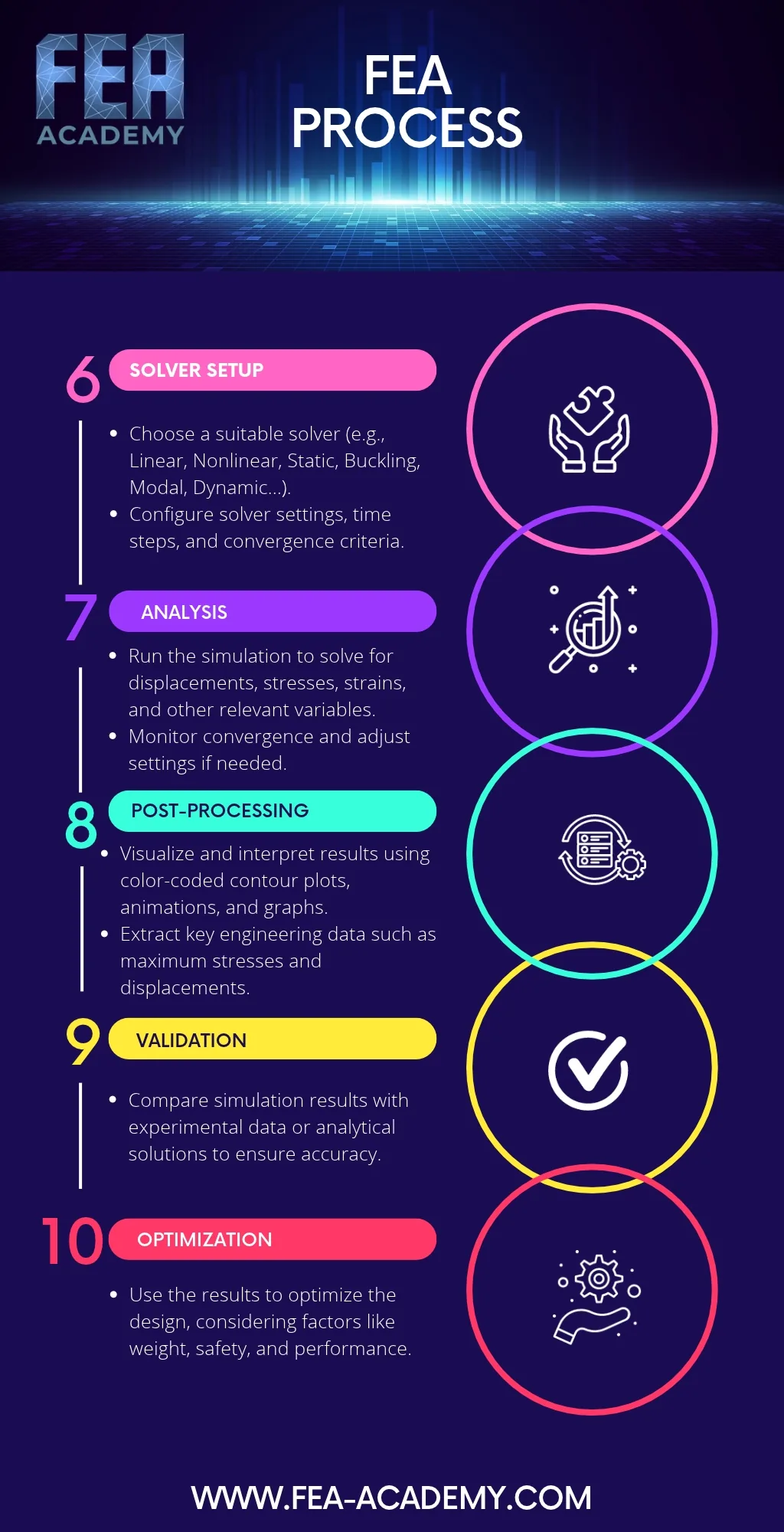
Choose a suitable solution type (linear, nonlinear, static, buckling, modal, dynamic). Configure the solver settings, time steps and convergence criteria.

The solution type must match the physics of the problem. A linear static solution assumes small displacements, linear elastic materials and contacts that do not change. If any of these assumptions is wrong, a nonlinear solution is needed. A linear buckling solution gives a critical load factor and a mode shape, but not the post-buckling behavior. A modal solution gives natural frequencies and mode shapes. A transient dynamic solution gives the response over time.

For nonlinear and dynamic solutions, the settings matter as much as the solution type:

• load increments and the maximum number of iterations;
• convergence criteria on forces, displacements or energy;
• time step size and damping for dynamic analyses;
• the number of modes and the frequency range for modal and frequency response analyses.

The default settings of the solver are a starting point, not a guarantee. They are designed to work reasonably for a wide range of problems, and they may not be appropriate for yours.

Step 7: Analysis

Run the simulation to solve for displacements, stresses, strains and other relevant variables. Monitor the convergence and adjust the settings if needed.

This is the step where the computer does the work. For a linear static analysis of a moderate model, it may take seconds. For a large nonlinear or dynamic analysis, it can take hours or days.

The engineer's role during the analysis is to monitor it. For nonlinear solutions, this means following the convergence history: how many iterations each increment needs, whether the increments are being cut back, and whether the solution is approaching the final load. A solution that needs more and more iterations, or smaller and smaller increments, is telling you something about the model: an instability, a contact that chatters, a material that softens, or a boundary condition that is missing.

When the run is complete, the solver output file must be read. Warnings about singularities, high stiffness ratios, distorted elements or negative pivots are early signs of a problem in the model. Ignoring them is a common way of reporting wrong results with confidence.

Step 8: Post-processing

Visualize and interpret the results using color-coded contour plots, animations and graphs. Extract the key engineering data, such as maximum stresses and displacements.

Post-processing turns millions of numbers into engineering information. It starts with plausibility checks, not with the maximum stress:

• Deformed shape: does the structure deform the way you expect? Animate it. Unexpected deformations usually reveal a missing constraint, a wrong load direction or an element connectivity problem.
• Reaction forces: do the reactions balance the applied loads? Are they distributed between the supports as expected?
• Order of magnitude: are the displacements and stresses consistent with the hand calculation made in step 1?

Only after these checks should you look at the detailed results. When you do, choose the result that matches your failure criterion: von Mises stress for ductile yielding, principal stresses for brittle materials and fatigue, specific components for composites. Be careful with averaged nodal stresses at material interfaces and at singularities, where averaging can hide or create peaks. Finally, extract the values needed for the decision, such as the maximum stress in each component, the margin of safety, or the displacement at a critical point.

Phase 3: checking and improving

Step 9: Validation

Compare the simulation results with experimental data or analytical solutions to ensure accuracy.

Validation answers the question: does the model represent reality? Verification checks that the equations are solved correctly; validation checks that the right equations are solved. Both are needed before a result can be trusted.

Validation can be performed at several levels:

• comparison with analytical solutions for simplified configurations, such as beam theory, plate formulas or classical stress concentration factors;
• comparison with benchmark problems that have known reference solutions;
• comparison with physical tests, from material coupons to components and complete structures, using strain gauges, displacement transducers or digital image correlation;
• comparison with previous analyses of similar structures that have been validated.

The level of validation should match the consequences of the decision. A quick concept study may only need a hand calculation for comparison. A safety-critical component may need a full test correlation program. When the model and the test disagree, the difference is information: it points to a boundary condition, a material property or an assumption that needs to be revisited.

Step 10: Optimization

Use the results to optimize the design, considering factors such as weight, safety and performance.

Once the model is validated, it becomes a tool for improving the design. This is where simulation brings much of its value: changing a thickness, a material or a shape in a model costs minutes, while changing a prototype costs weeks.

Optimization can be informal, with the engineer changing the design based on the stress distribution and the load paths, or formal, using optimization algorithms:

• sizing optimization adjusts parameters such as thicknesses and cross-sections;
• shape optimization modifies the boundaries of the part, such as fillet radii and contours;
• topography optimization finds the best pattern of beads and stiffeners in a shell;
• topology optimization finds the best distribution of material within a design space.

Whatever the method, the optimized design must be checked again. An optimizer will exploit every weakness of the model, so a design that is optimal for an inaccurate model may be poor in reality. The optimized configuration should go back through the relevant steps of the process, including validation.

Phase 4: delivering

Step 11: Documentation

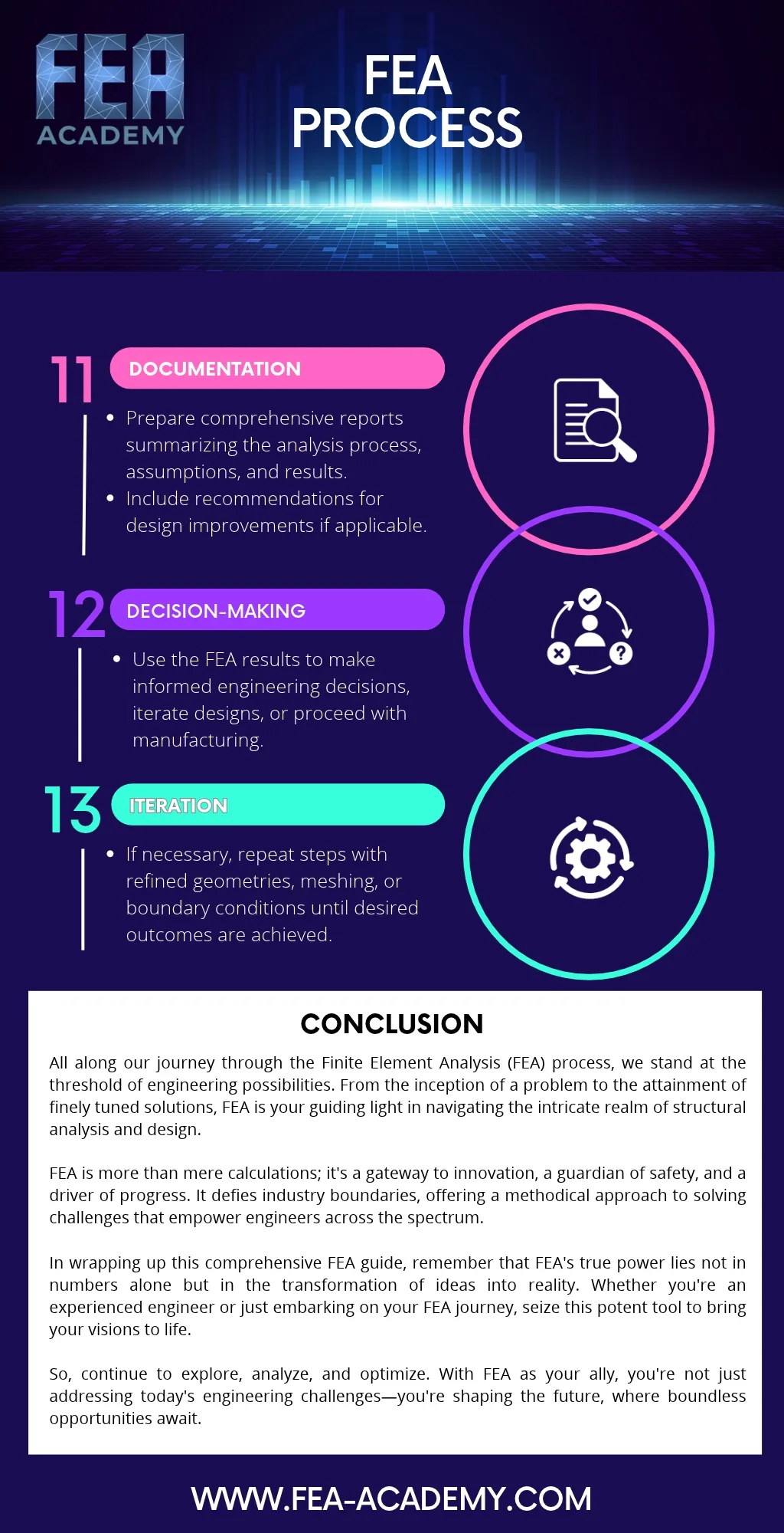
Prepare comprehensive reports summarizing the analysis process, assumptions and results. Include recommendations for design improvements if applicable.

An analysis that is not documented does not exist for anyone except its author, and even the author will forget the details within a few months. The FEA report is what allows others to understand, review, trust and reuse the work.

A good FEA report includes:

• the objective of the analysis and the questions it answers;
• the description of the model: geometry, idealizations, element types, mesh density and quality;
• the material properties and their sources;
• the boundary conditions and load cases;
• the assumptions, stated explicitly, with their justification;
• the verification checks: mesh convergence, reaction forces, hand calculations;
• the validation evidence, if any;
• the results, presented clearly with the relevant plots and tables;
• the conclusions and recommendations.

The report should allow a competent engineer to reproduce the analysis. The model files, input decks and results should be archived with the report, with clear version control.

Step 12: Decision-making

Use the FEA results to make informed engineering decisions, iterate designs, or proceed with manufacturing.

The purpose of every analysis is a decision. The design is acceptable, or it needs to be changed. Concept A is better than concept B. The failure was caused by this load case. The part can proceed to manufacturing.

Making a good decision from FEA results requires understanding their uncertainty. Results that are close to an acceptance limit deserve more scrutiny than results with large margins. The sensitivity of the result to the main assumptions, for example the stiffness of a joint or a material property, tells the decision-maker how robust the conclusion is. A good analyst presents the results with this context, not as a single number without qualification.

Step 13: Iteration

If necessary, repeat the steps with refined geometries, meshes or boundary conditions until the desired outcomes are achieved.

The FEA process is a loop, not a line. Validation may reveal a boundary condition that must be changed. Optimization produces a new design that must be analyzed. A design review asks for an additional load case. A test shows a behavior the model did not capture.

Each iteration should go back to the step where the change applies and follow the process forward from there. Changing a mesh requires a new convergence check. Changing a boundary condition requires new reaction force checks. Changing the design requires new validation if the change affects the validated behavior. Iteration is efficient when the earlier work was well documented, because each change can be made and checked in a controlled way.

Common pitfalls across the process

Looking at the process as a whole, a few pitfalls appear again and again:

• Starting with the mesh: jumping into the preprocessor before defining the problem leads to models that answer the wrong question or have the wrong level of detail.
• Trusting the defaults: element types, solver settings and convergence criteria have defaults for convenience, not for accuracy.
• Skipping the plausibility checks: going directly to the maximum stress without looking at the deformed shape and the reaction forces.
• Confusing verification and validation: a converged mesh does not prove that the model represents reality.
• Reporting without context: presenting a single number without its assumptions, its uncertainty and its sensitivity.

Conclusion

The finite element method is a powerful tool, but its power comes from the process around it. The thirteen steps described in this article, from problem definition to iteration, turn a piece of software into a reliable engineering method. They take an idea, test it in a virtual environment, check it against reality, improve it, and turn it into a documented decision.

Whether you are an experienced engineer or just starting your FEA journey, following a structured process is the most effective way to produce results that you and your colleagues can trust. The tools will keep changing. The process, and the engineering judgment behind each step, will remain the foundation of good analysis.

See all articles