
Every day, engineers around the world run millions of finite element analyses. They size aircraft wings, certify medical implants, crash cars that do not exist yet, and check that bridges, dams and offshore platforms will stand. For most of them, the finite element method is simply there, built into the software they open every morning. Yet the method is barely seventy years old, and its history is one of the most remarkable stories in engineering: an idea that appeared independently in applied mathematics, civil engineering and aeronautics, that was given its name by a professor during a summer job at an aircraft company, and that grew in a few decades into the universal language of structural analysis.
This article tells that story in full, from the variational principles of the eighteenth and nineteenth centuries to the machine learning methods of today. It follows the people, the problems and the computers that shaped the method, and it explains why each step mattered for the engineer who uses FEA now. References are given throughout and collected at the end for readers who want to go to the original sources.
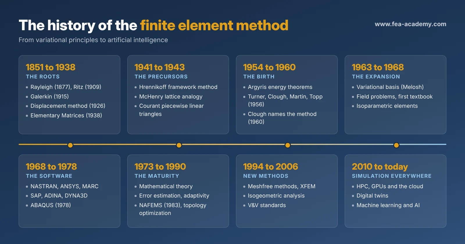
The roots: variational principles and approximate methods
The finite element method rests on an idea much older than the computer: that the state of equilibrium of a physical system is the one that makes a certain quantity, usually an energy, stationary. This idea comes from the calculus of variations, developed in the eighteenth century by Leonhard Euler and Joseph-Louis Lagrange. In structural mechanics it takes the form of the principle of minimum potential energy: among all the displacement fields that satisfy the supports, the one that actually occurs minimizes the total potential energy of the structure.
For most real problems, the exact minimizing function cannot be found. In the nineteenth and early twentieth centuries, mathematicians and physicists developed methods to approximate it.
Lord Rayleigh, in The Theory of Sound (1877), estimated the natural frequencies of vibrating systems by assuming a reasonable shape for the vibration mode and computing the corresponding energy [1]. The estimate was remarkably good, and it was always on the high side, a property that would later become important for the finite element method.
Walter Ritz, a Swiss physicist, generalized this idea in 1909 [2]. He proposed to approximate the unknown function as a combination of several known trial functions, each multiplied by an unknown coefficient, and to choose the coefficients that minimize the energy. The result is a system of algebraic equations in the coefficients. The Rayleigh-Ritz method is, in essence, the finite element method with trial functions defined over the whole domain instead of over small elements.
Ivan Bubnov (1913) and Boris Galerkin (1915) [3], Russian engineers working on plates and shells, proposed a related method that does not require an energy functional. It requires instead that the error of the approximate solution be orthogonal to the trial functions. The Galerkin method applies to a wider range of equations, including problems for which no energy principle exists, and it is the basis of most modern finite element formulations.
The weakness of these classical methods was the choice of the trial functions. For a simple shape, such as a rectangular plate, good functions can be found. For an irregular shape with holes and cutouts, finding functions that satisfy the boundary conditions over the whole domain is practically impossible. The decisive step of the finite element method would be to define simple trial functions over small pieces of the domain instead of complicated functions over the whole of it.
There were early hints of this step. In 1851, the German mathematician Karl Schellbach approximated a minimal surface by dividing it into triangles, an approach that historians of the method have identified as a remote ancestor of finite elements [4]. But without computers to solve the resulting equations, such ideas remained curiosities.
Matrix structural analysis before the computer
In parallel with the mathematicians, structural engineers developed their own methods for analyzing frameworks of bars and beams, the structures of bridges, roofs and buildings.
James Clerk Maxwell (1864), Alberto Castigliano (1879) and Otto Mohr laid the foundations of the force method, in which the unknowns are the internal forces of a statically indeterminate structure, found from the conditions of compatibility of displacements. In 1926, the Danish engineer Asger Ostenfeld formalized the displacement method, in which the unknowns are the displacements of the joints, found from the equilibrium of forces. These two methods, force and displacement, are the two faces of matrix structural analysis, and the displacement method is the direct ancestor of the finite element method used in most software today [5].
Before computers, the equations of large frameworks were solved by hand, often by iterative procedures. Hardy Cross's moment distribution method (1930) and Richard Southwell's relaxation methods (1930s and 1940s) allowed engineers to solve statically indeterminate structures with pencil and paper, by successive corrections. They were ingenious and widely used, but they were limited to problems of moderate size.
In aeronautics, where structures are light, thin-walled and highly indeterminate, the problem was more acute. The book Elementary Matrices by Frazer, Duncan and Collar (1938) introduced matrix algebra to the analysis of aircraft flutter and vibration, and prepared engineers to write their structural problems in matrix form [5]. When digital computers arrived, this matrix formulation would make the transition natural.
The 1940s: three independent precursors
The early 1940s saw three contributions that, with hindsight, contain the essential idea of finite elements. Their authors worked independently, in very different fields.
Hrennikoff and the framework method (1941)
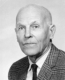
Alexander Hrennikoff, a Russian-born civil engineer working in Canada, proposed in 1941 to solve problems of plane elasticity by replacing the continuous material with a lattice of elastic bars arranged so that the lattice has the same stiffness as the continuum [6]. A plate became a framework, and the framework could be solved with the methods of structural analysis. This framework method discretized a continuous body into simple structural pieces, exactly the concept that the finite element method would later formalize.
McHenry and the lattice analogy (1943)
Two years later, Douglas McHenry, working on the stress analysis of concrete dams in the United States, published a similar lattice analogy [7]. Like Hrennikoff, he replaced the continuum with an equivalent arrangement of bars. Both methods worked, but they had a limitation: the lattice is an analogy, and finding a lattice that represents the continuum accurately for all loading conditions is difficult.
Courant and piecewise trial functions (1943)
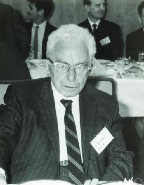
The third contribution came from pure mathematics. In May 1941, Richard Courant, a German mathematician who had emigrated to New York University, gave an address to the American Mathematical Society, published in 1943 [8]. Discussing the Saint-Venant torsion problem, he proposed to use the Rayleigh-Ritz method with trial functions that are linear over each triangle of a triangular mesh, and continuous from triangle to triangle. This is exactly the linear triangular finite element, described twelve years before engineers rediscovered it.
Courant's paper is often cited as the mathematical origin of the finite element method. At the time, however, it attracted little attention from engineers. Without computers, a method requiring the solution of hundreds of simultaneous equations had no practical future, and the mathematicians and engineers who would later meet were not yet talking to each other.
The 1950s: aeronautics gives birth to the method
The finite element method was finally born in the aircraft industry of the 1950s, out of necessity.
The problem: swept and delta wings
The jet age changed the shape of aircraft. Wings became thinner, swept back or triangular in plan form (the delta wing), and they carried large engines and fuel loads. The classical beam theory used to analyze straight wings, which treated the wing as a beam with a given stiffness, could not represent these low aspect ratio, highly redundant structures. Stiffness had to be known accurately, because it controlled flutter and aeroelastic behavior, phenomena that could destroy an aircraft in seconds.
Engineers such as Samuel Levy had already explored matrix methods for these structures [9]. At the same time, the first digital computers became available to the aircraft industry. The problem and the means to solve it arrived together.
The Boeing team: Turner, Clough, Martin and Topp
At the Boeing Airplane Company in Seattle, the head of the Structural Dynamics Unit was M. Jon Turner. Born in Oakville, Indiana, in 1915, Turner was a practical engineer with a very concrete problem: classical beam theory could not predict the vibration of the thin delta and swept wings that Boeing was studying, and without reliable stiffness data, flutter and aeroelastic behavior could not be predicted either [65].
To attack the problem, Turner brought academics into the company through a summer faculty program. In the summer of 1952, he hired Ray W. Clough, a young professor of structural engineering at the University of California, Berkeley, and Harold C. Martin, a professor at the University of Washington. Clough first tried to represent the wing skin with assemblies of beams, in the spirit of the framework method. The results did not match the tests, and Clough later described that first summer as a failure [10][11][66].
When Clough came back in 1953, Turner proposed a different approach: represent the skin of the wing with plate elements, triangles and rectangles connected to each other only at their corners, whose stiffness is derived directly from the theory of elasticity by assuming a simple displacement field inside each element. This time, the approach worked.
With Martin and L. J. Topp, a Boeing engineer, Turner and Clough presented the work in January 1954 at the annual meeting of the Institute of the Aeronautical Sciences in New York. The paper was published in September 1956 as "Stiffness and deflection analysis of complex structures" in the Journal of the Aeronautical Sciences [12].
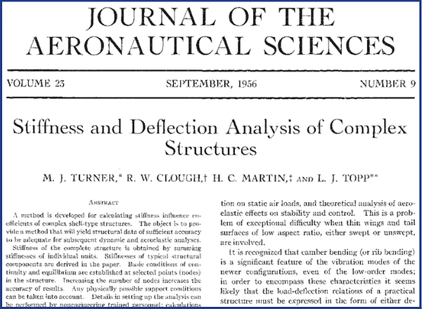
The paper described how to derive the stiffness of triangular and rectangular elements, how to assemble them into the stiffness matrix of the complete structure, and how to solve for the displacements. It is the founding document of the finite element method in engineering.
The method described in the 1956 paper is the direct stiffness method: each element has a stiffness matrix relating forces and displacements at its corner nodes, and the global stiffness matrix is assembled by adding the contributions of all the elements at the shared nodes. This procedure is still at the heart of every finite element program.
Turner designed the method from the start for computer implementation. Its steps are systematic and repetitive: compute the stiffness of each element, add it into the global matrix, apply the supports, solve. That is exactly what a computer does well, and it is why the direct stiffness method, rather than the many alternative formulations of the time, became the basis of finite element software. Turner also convinced Boeing's management to support the approach, and the company went on to apply it on a large scale, including in the development of the 747, which first flew in 1969 [65]. Turner died in 1995, at the age of 80 [67].
Argyris and the energy theorems
At the same time, in Europe, another engineer was reaching the same destination by a completely different road.
John Argyris was born Johann Hadjiargyris on 19 August 1913 in Volos, Greece. He graduated from the Technical University of Munich in 1936 and began his career in Germany on the design of guyed radio masts, slender structures in which the interaction of many members must be computed carefully. During the Second World War, he was imprisoned in Germany, escaped to Switzerland, and completed his doctoral studies at ETH Zurich before moving to England in 1943. He joined Imperial College London in 1949 and became a full professor there in 1955 [65][68][69].
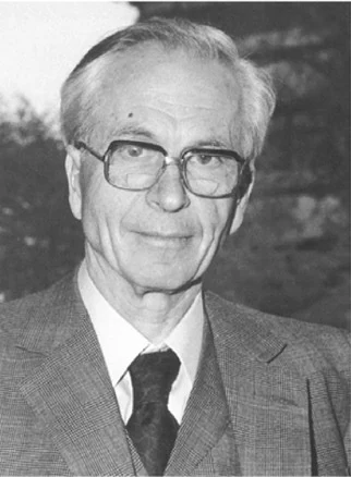
At Imperial College, Argyris developed a general and rigorous framework for matrix structural analysis. Between October 1954 and May 1955, he published a series of articles in the journal Aircraft Engineering titled "Energy theorems and structural analysis" [13]. They were later collected in a book with Sydney Kelsey (1960) [14].
Argyris showed how the energy principles of structural mechanics lead naturally to matrix formulations, and he demonstrated the duality between the force method and the displacement method. His work included the derivation of the stiffness of a rectangular panel, a forerunner of finite elements, and gave the matrix methods a theoretical foundation that was general enough to be programmed for any structure. In 1959, Argyris took a joint appointment at the University of Stuttgart, where his institute developed the ASKA finite element program, one of the first large general-purpose FE systems. He also founded the journal Computer Methods in Applied Mechanics and Engineering, which became one of the leading journals of the field. He was elected a Fellow of the Royal Society in 1986, and he died in Stuttgart on 2 April 2004, at the age of 90 [65][68].
Two roads to the same matrix: the forgotten fathers
Turner and Argyris arrived at the same result from opposite directions. Turner started from a specific engineering problem, the stiffness of a delta wing, and built a practical procedure that a computer could execute. Argyris started from a general principle, the energy theorems of structural mechanics, and derived from it a systematic matrix formulation valid for any structure. Carlos Felippa, in his history of matrix structural analysis, places both of them at the center of the transition from the matrix methods of the 1930s and 1940s to the finite element method [5].
Yet when engineers are asked who invented the finite element method, they usually name Ray Clough, and sometimes Richard Courant or Olgierd Zienkiewicz. Turner and Argyris are much less known. There are at least three reasons for this [65]:
- The name made the hero. Clough gave the method its name in 1960, and a name attracts history. The person who named the method became, in the collective memory, the person who invented it.
- Industrial pioneers do not write textbooks. Turner was an engineer at Boeing. He solved problems, built a method and moved on to the next aircraft. He did not write the textbooks and review papers that shape how a field remembers its origins.
- Argyris worked in difficult places for visibility. Part of his early work was carried out in a wartime context where publication was restricted, and his later work was largely done in Germany, outside the English-speaking academic networks that wrote most of the history of the method.
Recognizing Turner and Argyris does not diminish the contributions of Clough, Courant or Zienkiewicz. It completes the picture: the finite element method was not invented by one person, but by several people who, from different starting points, recognized that complex structures could be analyzed by assembling simple pieces. The full story of these two forgotten fathers is told in the Beyond the Mesh article The Two Forgotten Fathers of the Finite Element Method.
Computers make it practical
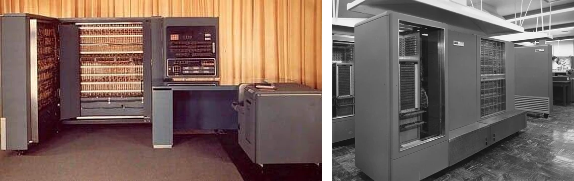
None of this would have mattered without computers. In the 1950s, machines such as the IBM 701 and 704 made it possible to solve systems of tens or hundreds of equations in a reasonable time. As the capacity of computers grew, so did the size of the structures that could be analyzed. The finite element method and the digital computer grew up together, and each pushed the other forward.
The 1960s: a name, a theory and an explosion
Clough names the method (1960)
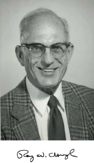
In 1960, Ray Clough presented a paper titled "The finite element method in plane stress analysis" at the second ASCE Conference on Electronic Computation in Pittsburgh [15]. It was the first time the name finite element method appeared in print. Clough chose the name to distinguish the finite pieces of the model from the infinitesimal elements of calculus. The name stuck.
The 1960 paper also marked a change of field. Clough applied the method to problems of civil engineering, such as the stresses in concrete dams, showing that the technique developed for aircraft wings was a general method for continuum mechanics. Back at Berkeley, Clough and his student and colleague Edward L. Wilson developed some of the first general-purpose finite element programs, which they distributed freely to other researchers and engineers.
The method finds its theoretical basis
At first, the finite element method was an engineering technique justified by intuition and by comparison with tests. In the early 1960s, several researchers showed that it was in fact a form of the Rayleigh-Ritz method applied with piecewise trial functions. Ray Melosh (1963) demonstrated that the displacement-based finite element method follows from the principle of minimum potential energy [16], and Jan Besseling and others reached similar conclusions. This link explained why the method converges as the mesh is refined, under certain conditions on the elements, and it reconnected the engineering work of the 1950s with the mathematics of Courant.
Once the method was understood as a variational method, it could be applied to any problem governed by a variational principle, not only to structures.
Zienkiewicz extends the method beyond structures
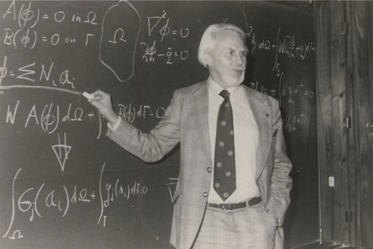
Olgierd C. Zienkiewicz, a Polish-born British engineer who became professor at the University of Wales in Swansea, played a decisive role in this extension. With his student Y. K. Cheung, he showed in 1965 that the finite element method could solve field problems such as heat conduction, seepage and electrical potential [17]. In 1967, they published The Finite Element Method in Structural and Continuum Mechanics [18], the first textbook devoted to the method. Through its successive editions, it became one of the most widely read books in engineering, and Swansea became one of the world centers of finite element research.
Zienkiewicz also co-founded, with Richard Gallagher, the International Journal for Numerical Methods in Engineering in 1969, which gave the growing community its own forum.
An independent discovery in China
The finite element method was also discovered independently in China. In the early 1960s, the mathematician Feng Kang and his group in Beijing, working on the design of the Liujiaxia dam, developed a systematic discretization method based on variational principles, published in 1965 [19]. Because of the political isolation of China at the time, this work remained unknown in the West for many years. It is now recognized as an independent creation of the finite element method, with a rigorous mathematical foundation.
The Wright-Patterson conferences
In 1965, the United States Air Force organized the first Conference on Matrix Methods in Structural Mechanics at Wright-Patterson Air Force Base in Ohio. This conference and the two that followed (1968 and 1971) brought together the pioneers of the method from the aerospace industry and universities. Many key ideas were first presented there, including new plate bending elements and the first form of the patch test, proposed by Bruce Irons and his colleagues as a practical check that an element will converge [20].
Better elements: the isoparametric revolution
The first elements were simple: constant strain triangles, rectangles and bars. They needed very fine meshes to give accurate results, and they could not represent curved boundaries. During the 1960s, researchers developed elements with more nodes and higher-order displacement fields.
The most important advance was the isoparametric element, introduced by I. C. Taig (1961) [21] and generalized by Bruce Irons (1966) [22] and by Ergatoudis, Irons and Zienkiewicz (1968) [23]. The idea is elegant: the same functions are used to describe the geometry of the element and the displacement field inside it. A quadrilateral element can then have curved sides, and its stiffness is computed by numerical integration (Gauss quadrature) on a reference square. Isoparametric elements are still the basis of most solid and shell elements in commercial software.
Other researchers explored alternative formulations: equilibrium models by Baudouin Fraeijs de Veubeke in Belgium, hybrid elements by Theodore Pian at MIT (1964), and mixed formulations that use both displacements and stresses as unknowns. Plate and shell bending elements, which require continuity of rotations between elements, proved particularly difficult, and the search for good plate and shell elements continued for decades.
Nonlinear and dynamic analysis begin
The 1960s also saw the first steps beyond linear static analysis:
- Geometric nonlinearity: Turner, Dill, Martin and Melosh (1960) analyzed large deflections of structures under heating and external loads [24].
- Material nonlinearity: Pedro Marcal and Ian King (1967) formulated elastic-plastic finite element analysis [25].
- Dynamics: John Archer (1963) introduced the consistent mass matrix [26], while time integration schemes such as Nathan Newmark's method (1959) [27] were adapted to finite element models. Robert Guyan (1965) proposed a method to reduce the size of models [28], and Roy Craig and Mervyn Bampton (1968) introduced component mode synthesis [29], still used today to analyze large dynamic systems.
By the end of the 1960s, the finite element method had become a general method for linear and nonlinear, static and dynamic, structural and field problems. What it needed now was software that engineers outside research centers could use.
The 1970s: the birth of the commercial programs
NASTRAN
In 1965, NASA launched a project to develop a general-purpose structural analysis program for the aerospace industry. The contract was won by a team including the MacNeal-Schwendler Corporation (MSC), founded in 1963 by Richard MacNeal and Robert Schwendler, together with Computer Sciences Corporation and the Martin Company [30]. The program, called NASTRAN (NASA Structural Analysis), was released to NASA in 1968 and to the public in 1971 through NASA's Office of Technology Utilization [31].
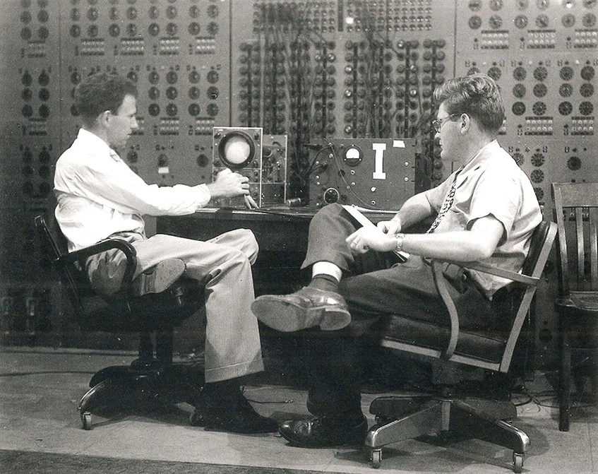
NASTRAN brought finite element analysis to the whole aerospace industry. Its input format, built around "bulk data" cards describing grid points, elements, properties and loads, became an industry standard that is still used today. In 1971, MSC released its own proprietary version, MSC/NASTRAN [30], which became the reference structural solver of the aerospace and automotive industries for decades.
ANSYS
In 1970, John Swanson, an engineer who had worked on the analysis of nuclear reactor components at Westinghouse, founded Swanson Analysis Systems in Pennsylvania [32]. His program, ANSYS, was designed as a general-purpose tool for engineers in all industries, with thermal, structural and later multi-physics capabilities. The company was renamed ANSYS, Inc. in 1994, and grew into one of the largest engineering simulation companies in the world.
MARC, SAP and ADINA
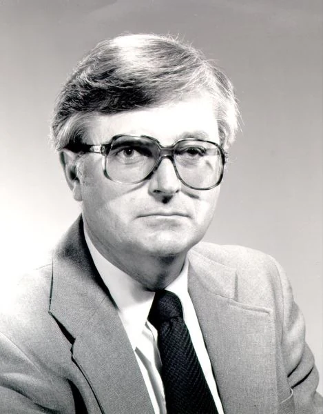
In 1971, Pedro Marcal founded the MARC Analysis Research Corporation, whose program MARC was the first commercial finite element code dedicated to nonlinear analysis. At Berkeley, Edward Wilson released the SAP program (Structural Analysis Program) in 1970 [33], freely distributed, which became the ancestor of many civil engineering programs. Klaus-Jürgen Bathe, a student of Wilson, developed ADINA (Automatic Dynamic Incremental Nonlinear Analysis) in 1975 at MIT, focused on nonlinear and dynamic problems.
Explicit dynamics: DYNA3D
In 1976, John Hallquist at Lawrence Livermore National Laboratory developed DYNA3D, an explicit finite element program for impact and high-speed dynamic problems [34]. Explicit methods avoid the solution of large systems of equations by advancing the solution in very small time steps, which makes them ideal for crash, impact and explosion simulations. Hallquist founded the Livermore Software Technology Corporation in 1987, and its commercial program LS-DYNA became the standard tool for automotive crash simulation.
ABAQUS
In 1978, David Hibbitt, Bengt Karlsson and Paul Sorensen, who had worked with Marcal, founded Hibbitt, Karlsson and Sorensen (HKS) and released ABAQUS, a program designed for advanced nonlinear analysis. ABAQUS became known for its robust handling of contact, plasticity and large deformations, and it became a reference in research and in industries such as automotive, tire, energy and biomedical engineering.
The working conditions of the time
Running FEA in the 1970s was very different from today. Models were described on punched cards, submitted to a mainframe computer, and the results came back hours or days later as printouts of numbers. There was no graphical pre-processing or post-processing at first; engineers drew their meshes by hand on paper and checked the results by reading tables. A model of a few thousand degrees of freedom was large. This discipline had one advantage: every node and every element was the result of a deliberate decision, and engineers knew their models in detail.
By the late 1970s, pre- and post-processors began to appear, with graphical terminals that allowed engineers to see their meshes and their results. Minicomputers such as the DEC VAX, to which MSC/NASTRAN was ported in 1978 [30], brought FEA closer to the engineering departments.
The 1970s and 1980s: the mathematics matures
While the software spread through industry, mathematicians built a rigorous theory of the method, which explained when and why it works.
Convergence and error analysis
Gilbert Strang and George Fix published An Analysis of the Finite Element Method in 1973 [35], one of the first books to give a complete mathematical treatment of the method. Ivo Babuška, Philippe Ciarlet [36], J. Tinsley Oden [37] and many others developed the theory of convergence, error bounds and stability.
A key result was the stability condition for mixed formulations, known as the inf-sup or Babuška-Brezzi condition (Babuška 1973 [38], Brezzi 1974 [39]). It explains why some combinations of displacement and pressure interpolations work for incompressible materials while others fail, and it guided the design of elements for incompressible and nearly incompressible problems.
Error estimation and adaptivity
Engineers had always asked: how accurate is my mesh? In 1978, Babuška and Werner Rheinboldt proposed a posteriori error estimates, computed from the finite element solution itself [40]. In 1987, Zienkiewicz and Jian Zhu introduced a simple and practical error estimator based on the difference between the computed stresses and a smoothed stress field [41]. These estimators made adaptive mesh refinement possible: the program refines the mesh automatically where the error is large.
The p-version of the finite element method, in which accuracy is improved by increasing the polynomial order of the elements instead of reducing their size, was analyzed by Babuška, Barna Szabó and I. Norman Katz in 1981 [42], and the combination of both strategies, the hp-version, gave exponential convergence for many problems.
Locking and its cures
Practitioners discovered that some elements become far too stiff in certain situations: thin shells in bending, nearly incompressible materials, slender beams. This phenomenon, called locking, led to a series of remedies. Reduced integration (Zienkiewicz, Taylor and Too, 1971) [43] relaxed the excessive stiffness but introduced spurious zero-energy modes, called hourglass modes, which in turn required hourglass control (Flanagan and Belytschko, 1981) [44]. Selective integration and the B-bar method (Hughes, 1980) [45], incompatible modes, assumed strain and enhanced strain formulations followed. The element formulations used in today's commercial codes are the result of these decades of work.
Benchmarks and quality
As FEA spread, the need for quality control became evident. In 1983, the National Agency for Finite Element Methods and Standards (NAFEMS) was founded in the United Kingdom to promote the safe and reliable use of finite element technology. NAFEMS published benchmark problems with reference solutions, which allowed users and vendors to check their software. In 1985, Richard MacNeal and Robert Harder published a standard set of problems to test the accuracy of elements [46]. NAFEMS later became an international association, and its publications on benchmarks, verification, validation and simulation governance are still a reference.
The great textbooks
The 1970s and 1980s also produced the textbooks that trained generations of engineers: Robert Cook's Concepts and Applications of Finite Element Analysis (1974), Bathe and Wilson's Numerical Methods in Finite Element Analysis (1976) [47], Bathe's Finite Element Procedures in Engineering Analysis (1982) [48], Thomas J. R. Hughes's The Finite Element Method: Linear Static and Dynamic Finite Element Analysis (1987) [49], and the successive editions of Zienkiewicz's book, later co-authored with Robert Taylor.
The 1980s and 1990s: FEA reaches every engineer
From mainframes to workstations and PCs
In the 1980s, engineering workstations and then personal computers made FEA accessible outside large companies and research centers. Graphical user interfaces replaced punched cards. Pre-processors such as PATRAN and I-DEAS, and later Altair HyperMesh (1990), allowed engineers to build complex meshes interactively and to visualize results in color. The colorful contour plot, now the emblem of FEA, became standard.
Automatic meshing and CAD integration
Building a mesh by hand was the main bottleneck of FEA. Automatic mesh generators, particularly for tetrahedral elements, transformed the workflow: the engineer could import a CAD geometry and obtain a solid mesh in minutes. Finite element tools were integrated directly into CAD software, making simulation available to design engineers, not only to analysis specialists.
This democratization had two sides. It made FEA a routine part of product development, which was a great progress. But it also made it possible to run an analysis without understanding the method, a concern that the pioneers themselves expressed and that remains relevant today.
New application domains
The capacity of computers allowed FEA to address problems that were previously out of reach:
- Crash simulation: in the late 1980s and 1990s, explicit codes such as LS-DYNA, PAM-CRASH and RADIOSS made virtual crash testing a standard part of automotive development.
- Structural optimization: the homogenization method of Martin Bendsøe and Noboru Kikuchi (1988) [50] launched topology optimization, which finds the best distribution of material within a design space. Commercial tools such as Altair OptiStruct brought it to industry in the 1990s.
- Fracture and damage: the virtual crack closure technique (Rybicki and Kanninen, 1977) [51] and cohesive zone models, building on the work of Hillerborg and colleagues (1976) [52], made it possible to simulate crack growth and delamination in metals and composites.
- Composites: layered shell and solid elements, failure criteria and progressive damage models supported the growing use of composite materials in aerospace.
The 1990s and 2000s: new methods and an industry that consolidates
Beyond the classical finite element method
Researchers kept pushing the limits of the method, and several new families of methods appeared:
- Meshfree methods, such as the element-free Galerkin method (Belytschko, Lu and Gu, 1994) [53] and the reproducing kernel particle method (Liu and colleagues, 1995), approximate the solution without a mesh, which helps for very large deformations and fragmentation.
- The extended finite element method (XFEM) (Belytschko and Black, 1999 [54]; Moës, Dolbow and Belytschko, 1999 [55]) enriches the elements with special functions so that cracks can grow through the mesh without remeshing.
- Peridynamics (Silling, 2000) [56] reformulates continuum mechanics with integral equations, which naturally handle cracks and discontinuities.
- Isogeometric analysis (Hughes, Cottrell and Bazilevs, 2005) [57] uses the same spline functions (NURBS) that describe the geometry in CAD to approximate the solution, aiming to close the gap between design and analysis.
- Multiscale methods link the behavior of the material at the micro scale, such as fibers and matrix in a composite, to the response of the structure.
Verification, validation and simulation governance
As simulation took on more responsibility in design and certification, the question of its credibility became central. In 2006, the American Society of Mechanical Engineers published its Guide for Verification and Validation in Computational Solid Mechanics (ASME V&V 10) [58], which formalized the concepts of verification (solving the equations right) and validation (solving the right equations). Organizations such as NAFEMS developed the notion of simulation governance: the processes, competencies and controls that ensure simulation results can be trusted.
Industry consolidation
The commercial landscape changed through a series of acquisitions. MSC acquired MARC in 1999 [30]. Dassault Systèmes acquired ABAQUS in 2005 and made it the core of its SIMULIA brand. ANSYS acquired many companies, including the fluid dynamics leader Fluent (2006) and, in 2019, Livermore Software Technology Corporation, the developer of LS-DYNA. MSC Software was acquired by Hexagon in 2017 [30]. At the same time, open-source codes such as Code_Aster, CalculiX and FEniCS gave engineers and researchers free alternatives.
The 2010s to today: simulation everywhere
High-performance computing, GPUs and the cloud
The size of finite element models has grown with computing power. Global models of complete aircraft with millions of degrees of freedom, detailed models with hundreds of millions, and thousands of load cases are now routine in large companies. Parallel solvers distribute the work across many processors, graphics processing units (GPUs) accelerate both explicit and implicit solutions, and cloud computing gives small companies access to computing resources that were once reserved for national laboratories.
Simulation-driven design and digital twins
Simulation has moved from checking designs to driving them. Optimization, design exploration and parametric studies are integrated into the design process. Additive manufacturing has made it possible to build the complex shapes produced by topology optimization. The concept of the digital twin, a simulation model connected to the data of a real product in service, extends simulation into operation and maintenance.
The arrival of artificial intelligence
The most recent chapter is the combination of finite element methods with machine learning. Physics-informed neural networks (Raissi, Perdikaris and Karniadakis, 2019) [59] train neural networks to satisfy the governing equations. Graph neural networks trained on mesh-based simulations, such as MeshGraphNets (Pfaff and colleagues, 2021) [60], learn to predict the results of simulations much faster than the solvers that generated the training data. Neural operators and surrogate models allow the rapid exploration of design spaces, and researchers are building hybrid methods that combine finite element formulations with neural networks [61]. Major software vendors now integrate AI-based tools trained on simulation data into their products.
These methods are promising, but they do not replace the physics. A surrogate model is only as good as the simulations it was trained on, and it is only reliable within the range of those simulations. The questions raised by the pioneers, about convergence, accuracy and validation, apply to these new tools with even more force.
A new wave of consolidation
The years 2025 and 2026 saw the largest transactions in the history of the simulation industry. Siemens completed the acquisition of Altair Engineering in March 2025, for about 10 billion US dollars [62]. Synopsys, the electronic design automation company, completed its acquisition of ANSYS in July 2025, for about 35 billion US dollars [63]. In February 2026, Cadence Design Systems completed the acquisition of Hexagon's design and engineering business, which includes MSC Nastran, Marc and Adams [64]. More than fifty years after their creation, NASTRAN, ANSYS and MARC are now part of groups whose roots are in electronics and industrial automation, a sign of how central simulation has become to the design of every kind of product.
A timeline of the finite element method
| Year | Milestone |
|---|---|
| 1851 | Schellbach approximates a minimal surface with triangles |
| 1877 | Rayleigh, The Theory of Sound: energy-based approximation of vibrations |
| 1909 | Ritz generalizes the method of trial functions |
| 1915 | Galerkin publishes his weighted residual method |
| 1926 | Ostenfeld formalizes the displacement method for frameworks |
| 1938 | Frazer, Duncan and Collar, Elementary Matrices |
| 1941 | Hrennikoff's framework method |
| 1943 | McHenry's lattice analogy; Courant's piecewise linear trial functions |
| 1954 to 1955 | Argyris, "Energy theorems and structural analysis" |
| 1956 | Turner, Clough, Martin and Topp: the direct stiffness method for triangular elements |
| 1960 | Clough introduces the name "finite element method" |
| 1963 | Melosh shows the variational basis of the method |
| 1965 | Zienkiewicz and Cheung extend FEM to field problems; Feng Kang's work in China; first Wright-Patterson conference |
| 1966 to 1968 | Isoparametric elements (Irons; Ergatoudis, Irons and Zienkiewicz) |
| 1967 | Zienkiewicz and Cheung publish the first FEM textbook |
| 1968 | NASTRAN released to NASA |
| 1970 | Swanson Analysis Systems founded (ANSYS); SAP released at Berkeley |
| 1971 | MSC/NASTRAN; MARC; NASTRAN released to the public |
| 1973 | Strang and Fix, An Analysis of the Finite Element Method |
| 1975 | ADINA |
| 1976 | DYNA3D at Lawrence Livermore National Laboratory |
| 1978 | ABAQUS; Babuška and Rheinboldt's a posteriori error estimates |
| 1983 | NAFEMS founded |
| 1987 | Zienkiewicz-Zhu error estimator; LSTC founded (LS-DYNA) |
| 1988 | Bendsøe and Kikuchi: topology optimization |
| 1994 | Element-free Galerkin method |
| 1999 | Extended finite element method (XFEM) |
| 2005 | Isogeometric analysis; Dassault Systèmes acquires ABAQUS |
| 2006 | ASME V&V 10 guide for computational solid mechanics |
| 2019 | Physics-informed neural networks |
| 2021 | Graph neural networks for mesh-based simulation |
| 2025 | Siemens acquires Altair; Synopsys acquires ANSYS |
| 2026 | Cadence acquires Hexagon's design and engineering business (MSC Nastran) |
What the history of FEA teaches the engineer of today
Looking back over these seventy years, a few lessons stand out for engineers who use FEA today.
Credit belongs to many people. The finite element method has no single inventor. Turner, Argyris, Clough, Courant, Zienkiewicz, Feng Kang and many others each brought an essential piece. Knowing who did what, and why, helps us understand the method and its assumptions.
The method was born from engineering problems. The finite element method did not come from a desire to write software. It came from the need to predict the stiffness of a delta wing, the stresses in a dam, the temperature in a reactor. Every analysis should still start from the engineering question, not from the mesh.
The pioneers understood their elements. Turner, Clough, Argyris, Irons and Zienkiewicz derived their elements by hand, and they knew exactly what each element could and could not represent. Many of the errors made today, such as using first-order tetrahedra in bending or ignoring locking, come from forgetting what the pioneers knew.
Theory and practice need each other. The engineering intuition of the 1950s and the mathematical rigor of the 1970s together made the method reliable. Convergence, stability, error estimation and the patch test are not academic details; they are the reasons we can trust the results.
Verification and validation have always been part of the method. The Boeing team compared their results with tests. NAFEMS was founded to promote benchmarks. Today's V&V standards formalize what good engineers have always done.
The tools change, the fundamentals remain. From punched cards to cloud computing, from hand-drawn meshes to automatic meshing, from mainframes to neural networks, the tools have changed beyond recognition. The fundamentals, the right element, the right mesh, realistic boundary conditions, reliable material data, and rigorous checking, are the same as in 1956.
Conclusion
The finite element method is the product of many minds working over more than a century: mathematicians who developed variational principles, structural engineers who built the matrix methods, aeronautical engineers who needed to analyze new wings, civil engineers who analyzed dams, mathematicians who proved convergence, and software developers who made the method available to every engineer. Its history shows a rare combination of practical need, theoretical depth and computational power.
Today, the method continues to evolve, with new formulations, faster computers and artificial intelligence. Understanding where it comes from is one of the best ways to understand what it does, and to use it with the judgment that its pioneers brought to their work.
References
- Rayleigh, J. W. S. (1877). The Theory of Sound. London: Macmillan.
- Ritz, W. (1909). Über eine neue Methode zur Lösung gewisser Variationsprobleme der mathematischen Physik. Journal für die reine und angewandte Mathematik, 135, 1–61.
- Galerkin, B. G. (1915). Rods and plates: series in some questions of elastic equilibrium of rods and plates. Vestnik Inzhenerov i Tekhnikov, 19, 897–908 (in Russian).
- Williamson, F. (1980). A historical note on the finite element method. International Journal for Numerical Methods in Engineering, 15(6), 930–934.
- Felippa, C. A. (2001). A historical outline of matrix structural analysis: a play in three acts. Computers & Structures, 79(14), 1313–1324.
- Hrennikoff, A. (1941). Solution of problems of elasticity by the framework method. Journal of Applied Mechanics, 8(4), A169–A175.
- McHenry, D. (1943). A lattice analogy for the solution of stress problems. Journal of the Institution of Civil Engineers, 21(2), 59–82.
- Courant, R. (1943). Variational methods for the solution of problems of equilibrium and vibrations. Bulletin of the American Mathematical Society, 49(1), 1–23.
- Levy, S. (1953). Structural analysis and influence coefficients for delta wings. Journal of the Aeronautical Sciences, 20(7), 449–454.
- Clough, R. W. (1990). Original formulation of the finite element method. Finite Elements in Analysis and Design, 7(2), 89–101.
- Clough, R. W. (2004). Early history of the finite element method from the view point of a pioneer. International Journal for Numerical Methods in Engineering, 60(1), 283–287.
- Turner, M. J., Clough, R. W., Martin, H. C., & Topp, L. J. (1956). Stiffness and deflection analysis of complex structures. Journal of the Aeronautical Sciences, 23(9), 805–823.
- Argyris, J. H. (1954–1955). Energy theorems and structural analysis. Aircraft Engineering, 26 and 27 (series of articles).
- Argyris, J. H., & Kelsey, S. (1960). Energy Theorems and Structural Analysis. London: Butterworths.
- Clough, R. W. (1960). The finite element method in plane stress analysis. Proceedings of the 2nd ASCE Conference on Electronic Computation, Pittsburgh, PA.
- Melosh, R. J. (1963). Basis for derivation of matrices for the direct stiffness method. AIAA Journal, 1(7), 1631–1637.
- Zienkiewicz, O. C., & Cheung, Y. K. (1965). Finite elements in the solution of field problems. The Engineer, 220, 507–510.
- Zienkiewicz, O. C., & Cheung, Y. K. (1967). The Finite Element Method in Structural and Continuum Mechanics. London: McGraw-Hill.
- Feng, K. (1965). Finite difference schemes based on variational principles. Applied and Computational Mathematics, 2(4), 238–262 (in Chinese).
- Bazeley, G. P., Cheung, Y. K., Irons, B. M., & Zienkiewicz, O. C. (1965). Triangular elements in plate bending: conforming and non-conforming solutions. Proceedings of the Conference on Matrix Methods in Structural Mechanics, Wright-Patterson Air Force Base, Ohio, 547–576.
- Taig, I. C. (1961). Structural analysis by the matrix displacement method. English Electric Aviation Report S017.
- Irons, B. M. (1966). Engineering applications of numerical integration in stiffness methods. AIAA Journal, 4(11), 2035–2037.
- Ergatoudis, J., Irons, B. M., & Zienkiewicz, O. C. (1968). Curved, isoparametric, "quadrilateral" elements for finite element analysis. International Journal of Solids and Structures, 4(1), 31–42.
- Turner, M. J., Dill, E. H., Martin, H. C., & Melosh, R. J. (1960). Large deflections of structures subjected to heating and external loads. Journal of the Aerospace Sciences, 27(2), 97–107.
- Marcal, P. V., & King, I. P. (1967). Elastic-plastic analysis of two-dimensional stress systems by the finite element method. International Journal of Mechanical Sciences, 9(3), 143–155.
- Archer, J. S. (1963). Consistent mass matrix for distributed mass systems. Journal of the Structural Division, ASCE, 89(4), 161–178.
- Newmark, N. M. (1959). A method of computation for structural dynamics. Journal of the Engineering Mechanics Division, ASCE, 85(3), 67–94.
- Guyan, R. J. (1965). Reduction of stiffness and mass matrices. AIAA Journal, 3(2), 380.
- Craig, R. R., & Bampton, M. C. C. (1968). Coupling of substructures for dynamic analyses. AIAA Journal, 6(7), 1313–1319.
- NAFEMS. Analysis origins: MSC and NASTRAN. nafems.org
- Nastran. Wikipedia. en.wikipedia.org/wiki/Nastran
- CADFEM. 50 years of ANSYS: the early years, from 1970 to 1994. cadfem.net
- Wilson, E. L. (1970). SAP: A General Structural Analysis Program. Report UC SESM 70-20, University of California, Berkeley.
- Hallquist, J. O. (1976). Preliminary User's Manual for DYNA3D and DYNAP. Lawrence Livermore National Laboratory.
- Strang, G., & Fix, G. J. (1973). An Analysis of the Finite Element Method. Englewood Cliffs, NJ: Prentice-Hall.
- Ciarlet, P. G. (1978). The Finite Element Method for Elliptic Problems. Amsterdam: North-Holland.
- Oden, J. T. (1972). Finite Elements of Nonlinear Continua. New York: McGraw-Hill.
- Babuška, I. (1973). The finite element method with Lagrangian multipliers. Numerische Mathematik, 20(3), 179–192.
- Brezzi, F. (1974). On the existence, uniqueness and approximation of saddle-point problems arising from Lagrangian multipliers. RAIRO Analyse Numérique, 8(R2), 129–151.
- Babuška, I., & Rheinboldt, W. C. (1978). Error estimates for adaptive finite element computations. SIAM Journal on Numerical Analysis, 15(4), 736–754.
- Zienkiewicz, O. C., & Zhu, J. Z. (1987). A simple error estimator and adaptive procedure for practical engineering analysis. International Journal for Numerical Methods in Engineering, 24(2), 337–357.
- Babuška, I., Szabó, B. A., & Katz, I. N. (1981). The p-version of the finite element method. SIAM Journal on Numerical Analysis, 18(3), 515–545.
- Zienkiewicz, O. C., Taylor, R. L., & Too, J. M. (1971). Reduced integration technique in general analysis of plates and shells. International Journal for Numerical Methods in Engineering, 3(2), 275–290.
- Flanagan, D. P., & Belytschko, T. (1981). A uniform strain hexahedron and quadrilateral with orthogonal hourglass control. International Journal for Numerical Methods in Engineering, 17(5), 679–706.
- Hughes, T. J. R. (1980). Generalization of selective integration procedures to anisotropic and nonlinear media. International Journal for Numerical Methods in Engineering, 15(9), 1413–1418.
- MacNeal, R. H., & Harder, R. L. (1985). A proposed standard set of problems to test finite element accuracy. Finite Elements in Analysis and Design, 1(1), 3–20.
- Bathe, K. J., & Wilson, E. L. (1976). Numerical Methods in Finite Element Analysis. Englewood Cliffs, NJ: Prentice-Hall.
- Bathe, K. J. (1982). Finite Element Procedures in Engineering Analysis. Englewood Cliffs, NJ: Prentice-Hall.
- Hughes, T. J. R. (1987). The Finite Element Method: Linear Static and Dynamic Finite Element Analysis. Englewood Cliffs, NJ: Prentice-Hall.
- Bendsøe, M. P., & Kikuchi, N. (1988). Generating optimal topologies in structural design using a homogenization method. Computer Methods in Applied Mechanics and Engineering, 71(2), 197–224.
- Rybicki, E. F., & Kanninen, M. F. (1977). A finite element calculation of stress intensity factors by a modified crack closure integral. Engineering Fracture Mechanics, 9(4), 931–938.
- Hillerborg, A., Modéer, M., & Petersson, P. E. (1976). Analysis of crack formation and crack growth in concrete by means of fracture mechanics and finite elements. Cement and Concrete Research, 6(6), 773–781.
- Belytschko, T., Lu, Y. Y., & Gu, L. (1994). Element-free Galerkin methods. International Journal for Numerical Methods in Engineering, 37(2), 229–256.
- Belytschko, T., & Black, T. (1999). Elastic crack growth in finite elements with minimal remeshing. International Journal for Numerical Methods in Engineering, 45(5), 601–620.
- Moës, N., Dolbow, J., & Belytschko, T. (1999). A finite element method for crack growth without remeshing. International Journal for Numerical Methods in Engineering, 46(1), 131–150.
- Silling, S. A. (2000). Reformulation of elasticity theory for discontinuities and long-range forces. Journal of the Mechanics and Physics of Solids, 48(1), 175–209.
- Hughes, T. J. R., Cottrell, J. A., & Bazilevs, Y. (2005). Isogeometric analysis: CAD, finite elements, NURBS, exact geometry and mesh refinement. Computer Methods in Applied Mechanics and Engineering, 194(39–41), 4135–4195.
- ASME (2006). Guide for Verification and Validation in Computational Solid Mechanics (ASME V&V 10-2006). New York: American Society of Mechanical Engineers.
- Raissi, M., Perdikaris, P., & Karniadakis, G. E. (2019). Physics-informed neural networks. Journal of Computational Physics, 378, 686–707.
- Pfaff, T., Fortunato, M., Sanchez-Gonzalez, A., & Battaglia, P. W. (2021). Learning mesh-based simulation with graph networks. International Conference on Learning Representations (ICLR).
- Liu, W. K., Li, S., & Park, H. S. (2022). Eighty years of the finite element method: birth, evolution, and future. Archives of Computational Methods in Engineering, 29, 4431–4453. arxiv.org/abs/2107.04960
- NAFEMS. Siemens completes $10 billion acquisition of Altair Engineering. nafems.org
- Evertiq (2025). Synopsys completes $35 billion acquisition of Ansys. evertiq.com
- Evertiq (2026). Cadence completes acquisition of Hexagon's design and engineering business. evertiq.com
- Madier, D. (2026). The two forgotten fathers of the finite element method. Beyond the Mesh, FEA Academy. beyond-the-mesh.fea-academy.com
- Clough, R. W., & Wilson, E. L. (1999). Early finite element research at Berkeley. Proceedings of the 5th U.S. National Conference on Computational Mechanics, Boulder, CO.
- The Seattle Times (1995). Jonathan Turner, airplane engineer (obituary).
- National Academy of Engineering (2011). John H. Argyris 1913–2004. Memorial Tributes, Volume 15. Washington, DC: The National Academies Press.
- Kurrer, K.-E. (2018). The History of the Theory of Structures: Searching for Equilibrium (2nd ed.). Berlin: Ernst & Sohn.
Further reading on the history of the method: Zienkiewicz, O. C. (2004), The birth of the finite element method and of computational mechanics, International Journal for Numerical Methods in Engineering, 60(1), 3–10; Gupta, K. K., & Meek, J. L. (1996), A brief history of the beginning of the finite element method, International Journal for Numerical Methods in Engineering, 39(22), 3761–3774; Oden, J. T. (1990), Historical comments on finite elements, in S. G. Nash (ed.), A History of Scientific Computing, ACM Press, 152–166.
Go further
Learn FEA with a structured path: the on-demand course Practical Basic FEA covers the fundamentals step by step, and Practical Finite Element Analysis for Mechanical Engineers by Dominique Madier gathers the best modeling practices in one book.
See the Practical Basic FEA course Take the free FEA diagnostic