
Finite element analysis (FEA) is the most widely used simulation tool in mechanical and structural engineering. It lets engineers predict how a part, an assembly or a complete aircraft will respond to forces, pressure, temperature and vibration long before anything is manufactured. Yet many engineers use FEA software every day without a clear picture of what the method does behind the buttons. This article starts from the beginning: the three ways of solving an engineering problem, the numerical methods available, the partial differential equations that govern physics, and finally the idea at the heart of FEA, which is to divide a complex structure into simple pieces that a computer can solve.


Engineering simulation: a definition
Before defining FEA itself, it helps to place it in its wider family. According to NAFEMS, the International Association for the Engineering Modeling, Analysis and Simulation Community, engineering simulation is:
"the use of numerical, physical or logical models of systems and scientific problems in predicting their response to different physical conditions."
Three words in this definition deserve attention. The first is models: simulation never works on the real object, only on a representation of it. The second is predicting: the purpose of a simulation is to anticipate a behavior before it happens. The third is response: we are always interested in how a system reacts to something applied to it. FEA is one specific kind of numerical model, and everything that follows in this article is a consequence of this definition.
Three methods for solving an engineering problem
When engineers need to know whether a structure will carry its loads, they can choose among three families of methods: classical methods, numerical methods and experimental methods. Each one has its place, and a good analyst knows when to use which.
Classical methods
Classical methods are based on closed-form solutions. In structural engineering, they include the strength of materials and the theory of elasticity: the formulas you learned for the deflection of a cantilever beam, the stress in a simply supported plate or the torsion of a circular shaft. When they apply, they give accurate results and they are fast.
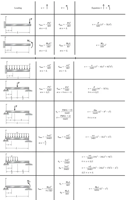
Their limitation is severe, though. Classical methods are only applicable to very simple problems: a cantilever beam, a simply supported plate, the torsion of a simple section, and similar textbook cases. They were used intensively at the beginning of the twentieth century, but today they are reserved for structures with simple geometry, loading and boundary conditions.
The weakness of these methods is that the engineer must make many reductive assumptions to force a complex situation into the framework of the equations. A real bracket with fillets, holes, bolted connections and a nonuniform load does not look like a textbook beam. To use a closed-form formula, you must simplify the geometry, idealize the supports and smooth the loads, and every simplification moves the answer further from reality. Real-world problems involve complex shapes, boundary conditions and material behaviors that classical methods simply cannot handle. This is why numerical methods were developed.
Numerical methods
Numerical methods produce mathematical representations of real-life engineering problems so that complex problems can be solved. They also rely on assumptions, but those assumptions are much less reductive than the ones required by classical methods. In other words, the assumptions of numerical methods are closer to reality.

Numerical methods give approximate solutions, not exact ones. With the advent of powerful computers, however, they have proven increasingly accurate and reliable, and today they are the standard way of analyzing complex structures in the automotive, aerospace, energy, medical and civil engineering industries.
Experimental methods
Experimental methods are based on measurements performed on a physical prototype. Strain gauges, displacement sensors and accelerometers record how the real object behaves under real loads. These methods are reliable and trusted, but they are time-consuming and expensive, and several specimens must usually be tested to obtain statistically meaningful results.

Experimental methods remain essential, because they are the reference used to validate numerical models. A finite element model correlated against test data is far more credible than one that was never compared with reality.
Classical versus numerical methods
The table below summarizes the differences between the two analytical approaches.
| Classical methods | Numerical methods | |
|---|---|---|
| Equations | Exact | Exact |
| Solutions | Exact | Approximate |
| Number of solutions | A few standard cases | All problems |
| Shapes, boundary conditions, loading | Simplifying assumptions | Treated as they are, without simplifying assumptions |
| Material | Only isotropic, only one material | All types of property, unlimited number of materials |
The key line is the third one. Classical methods give exact answers to a handful of idealized problems, while numerical methods give approximate answers to virtually any problem. For an engineer facing a real design, an approximate answer to the right problem is far more useful than an exact answer to the wrong one.
The pros and cons of physical prototyping
Prototyping deserves a closer look, because the choice between building and simulating is a daily decision in product development.
| Pros of prototyping | Cons of prototyping |
|---|---|
| Reliable | Very expensive compared with FEA |
| Well mastered | Time-consuming |
| Trusted by regulatory agencies | Degrades the competitiveness of products by raising design costs |
| Essential for the calibration and correlation of finite element models | Data integrity more difficult to maintain than with FEA |
| Cannot replicate all the conditions and environments the product will encounter during its life |
In modern product development, the two approaches are complementary. FEA is used to explore and refine designs quickly and at low cost, and testing is used to confirm the final design and to calibrate the models.
The four main numerical methods
Four numerical methods are commonly used to solve engineering problems. All of them can, in principle, be applied to the same problem, but they differ substantially in accuracy, ease of programming and computing time.
| Method | Typical use and limitations |
|---|---|
| Finite element method (FEM) | Used to solve complex mechanical problems. For structural analysis, it is by far the best method in terms of accuracy and computing time. |
| Boundary element method (BEM) | Considers only the outer boundaries of the domain, so it gives poor results when internal details, such as the stresses inside a part, are required. |
| Finite volume method (FVM) | Can be used for stress problems, but it is preferably used to solve computational fluid dynamics (CFD) problems. |
| Finite difference method (FDM) | Gives poor results with complicated geometry, assemblies of different materials and combinations of 1D, 2D and 3D elements. |
These four methods share a common point: they all approximate the solution of the partial differential equations (PDEs) that govern physics. To understand what FEA does, we therefore need a short reminder about PDEs.
A short introduction to partial differential equations
A differential equation is a mathematical equation that relates a function to its derivatives. Differential equations are used in almost every field of science and engineering: mechanics, heat transfer, fluid flow, electromagnetism, acoustics and many more. They link functions that represent physical quantities, such as displacement, temperature or pressure, to their derivatives, which represent the rates of variation of those same quantities.
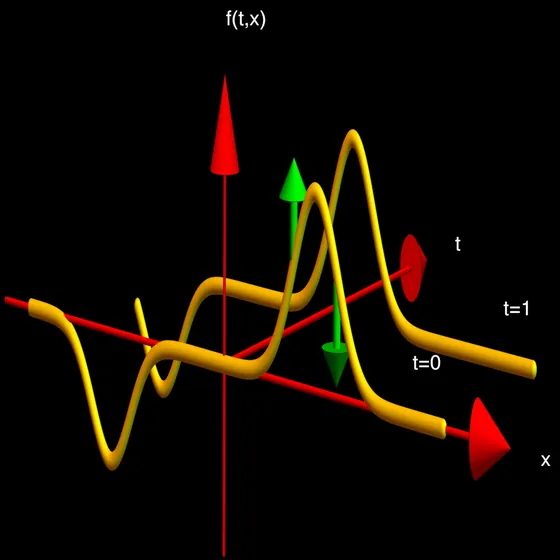
From a mathematical point of view, a PDE formulates phenomena described by functions of several variables. The temperature in a plate, for example, depends on the position x and on the time t. The equation is then made up of multivariable functions and their partial derivatives. A partial derivative of a function of several variables is its derivative with respect to one of those variables, with the others held constant: the change in temperature caused by a small change in time at a fixed position, or by a small change in position at a fixed time.
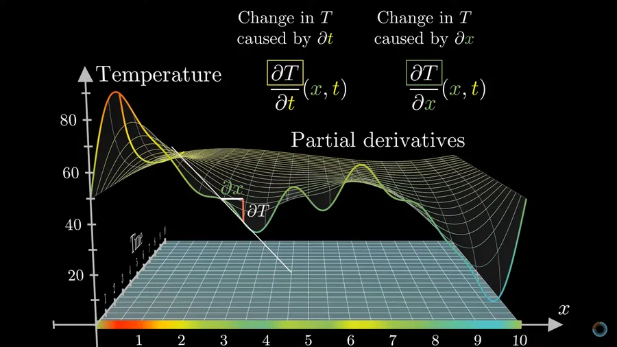
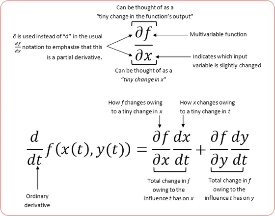
Here is the difficulty. While all physical problems can be expressed mathematically as differential equations, only the simplest ones can be solved with closed-form expressions, that is, mathematical expressions that can be evaluated in a finite number of operations. Many differential equations have no closed-form solution at all.
It is still possible, however, to find a solution to a differential equation without determining its exact form. When a closed-form solution is not available, the solution can be approximated numerically with a computer. This is exactly why numerical methods were developed: to determine solutions with a known and controllable degree of accuracy.
Why engineers need analysis and modeling
The need for analysis
Every real structure is characterized by its geometry, its materials, its properties and its boundary conditions. It is subjected to excitations, such as forces, pressure, accelerations, thermal effects and vibrations, and it produces a response in the form of displacements, forces, stresses, strains and natural frequencies.

The FEA analyst must determine the response of the structure under the given excitations in order to ensure that the structure can sustain them. Analysis serves design: we analyze so that we can design with confidence.
The need for modeling
The continuum nature of the problem and of its governing equations means that the real structure cannot be analyzed as it is. Only a model of the structure can be analyzed by a computer. The analyst therefore needs a tool to model the structure and to analyze the model.
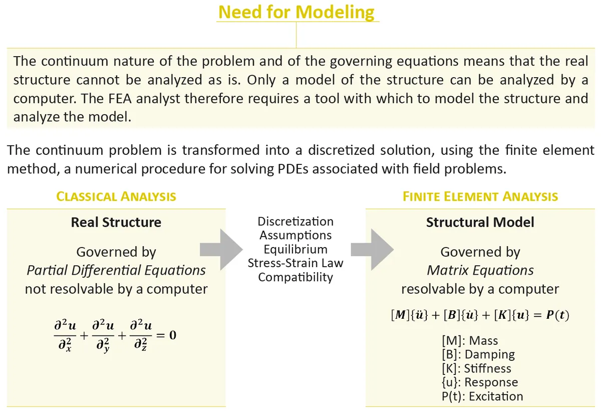
The finite element method provides this tool. It transforms the continuum problem into a discretized one: the real structure, governed by partial differential equations that a computer cannot solve directly, becomes a structural model governed by matrix equations that a computer can solve. The transformation relies on discretization, on modeling assumptions, and on three fundamental principles of mechanics: equilibrium, the stress-strain law and compatibility.
In structural analysis, the domain of interest is solid mechanics. The field variables are the displacements, which are the dependent variables governed by the differential equations. The boundary conditions are the specified values of the displacements at the limits of the analyzed system.
The equation at the heart of structural FEA
In solid mechanics, the finite element method is based on a matrix equation that defines the state of equilibrium of the forces acting on the structure:
[M]{ü} + [B]{u̇} + [K]{u} = P(t)
In this equation, [M] is the mass matrix, [B] is the damping matrix, [K] is the stiffness matrix, {u} is the vector of nodal displacements (with its first and second time derivatives, the velocities and accelerations), and P(t) is the excitation applied to the structure.
The most common analysis types are particular forms of this general equation:
| Analysis type | Governing equation |
|---|---|
| Linear static analysis | [K]{u} = P |
| Vibration (modal) analysis | ([K] − λ[M]){φ} = 0 |
| Linear buckling analysis | ([K] + λ[Kd]){φ} = 0 |
| Transient and frequency response analysis | [M]{ü} + [B]{u̇} + [K]{u} = P(t) |
Here λ is the ith eigenvalue, {φ} is the ith eigenvector, and [Kd] is the differential stiffness matrix, also called the geometric stiffness matrix. In a static analysis, the loads are applied slowly enough for the inertia and damping terms to vanish, so only the stiffness remains. In a modal analysis, there is no external load, and the solver looks for the natural frequencies and mode shapes of the structure. In a buckling analysis, it looks for the load factor at which the structure becomes unstable. Understanding which terms of the general equation are active in your analysis is one of the first steps toward choosing the right solution.
So, what is FEA? Divide and conquer
You may not be able to determine directly how a complex structural part will behave, but you can do so for a small and simple piece of it. FEA is built on this idea, which can be summarized in three words: divide and conquer.

If you divide a structure into many small elements, the behavior of each individual element provides a good approximation of the local behavior of the structure: its displacements, strains and stresses.
Discretization, or meshing
To run a simulation, the analyst creates a mesh made of small elements, sometimes millions of them, that together form the shape of the structure. This operation is called discretization or meshing. Calculations are made for every single element, and combining the individual results gives the behavior of the complete structure or system.

Nodes and interpolation
The results are obtained at certain points of the structure, but not at every point. These points are the nodes, located at the boundaries of the elements. Between the nodes, the way the field variable changes across each element is described by interpolation with polynomials, which can be linear, quadratic, cubic and so on. The order of these polynomials, together with the size of the elements, controls how accurately the model can represent a varying stress or displacement field.
Assembling the elements
The global assembly of all the individual elements reflects the behavior of the real structure. If you assemble enough of these simple pieces, you can determine how a complex structural part will behave. Mathematically, the solver assembles the equations of all the elements into one large matrix equation, which it then solves for the unknown nodal displacements.

A good discretization is a matter of balance
The more elements you use to represent your structure, the more precise and realistic the response you will get. But nothing is free: the more elements you use, the greater the computing time needed to solve the model.

A smaller mesh density gives less accuracy, less complexity and less computing time. A greater mesh density gives greater accuracy, more complexity and more computing time. The skill of the analyst lies in placing the elements where they are needed, with a fine mesh in the regions of high stress gradient and a coarser mesh elsewhere. The mesh convergence study is the tool used to verify that the mesh is fine enough in the critical regions.
From a continuous system to a discrete system
The key term in FEA is discretization: it transforms a continuum problem into a discretized solution.
- The continuous system (reality) is defined by an infinite number of points and governed by an infinite number of equations.
- The discrete system (the model) is defined by a finite number of nodes and governed by a finite number of equations.

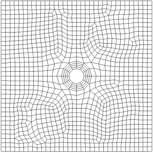
A few examples show how this works in practice. The simplest is a square plate, 100 inches by 100 inches, with a central hole, loaded in tension by 1,000 lb. It can be discretized with a two-dimensional mesh of quadrilateral elements, refined around the hole where the stress concentration occurs.
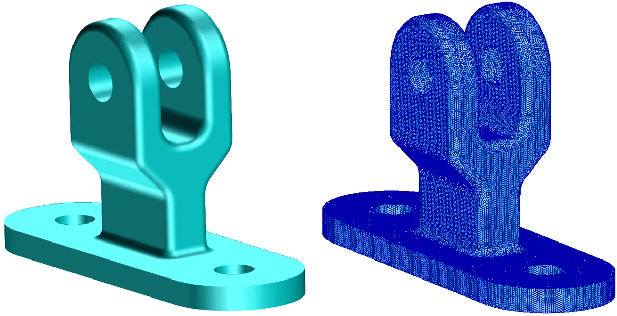
A machined fitting is a three-dimensional part, so it is discretized with solid elements. The CAD geometry on the left becomes the solid mesh on the right, and a closer look shows how the elements follow the holes and fillets of the part.
At the other end of the scale, a complete aircraft can be represented by a global finite element model (GFEM). Such a model is used to capture the global structural behavior of the aircraft and to compute the distribution of internal loads. With the skin removed, the internal structure of frames, stringers, floor beams and ribs becomes visible, and you can see how much detail such a model can contain.

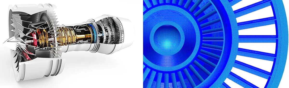
The same approach applies to an entire turbofan engine, with its fan, compressor, combustor and turbine stages, each represented by thousands of elements.
The four key words of finite element analysis
To summarize what FEA is, let us take its name word by word.
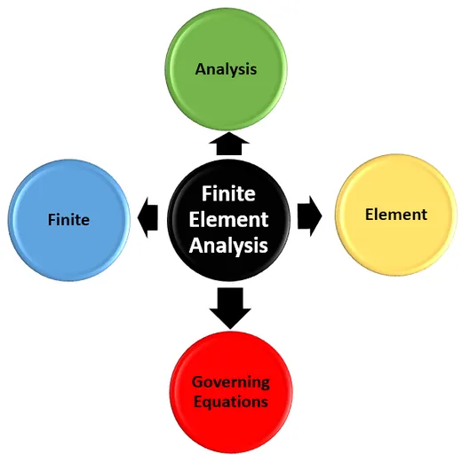
- Element: a small section of the analyzed part. Each element acts on its neighboring elements. FEA assembles the equations of all the elements into one large matrix equation, and the numerical solution is determined by a computer.
- Governing equations: the equations that describe how each element behaves. FEA solves them for the analyzed part depending on how it is held and loaded. The key concept of FEA is that, if the elements are small enough and are spread intelligently across the part, the numerical solution can closely approximate reality.
- Finite: the structure is represented by a countable number of elements, each of finite and measurable size.
- Analysis: the part is analyzed under specific conditions: static, dynamic, modal, buckling, linear or nonlinear.
Key takeaways
- Engineers can solve problems with classical, numerical or experimental methods. Classical methods are exact but limited to simple cases, experiments are reliable but costly, and numerical methods solve almost any problem with an approximate answer.
- Among the numerical methods, the finite element method is the reference for structural analysis.
- FEA approximates the solution of the partial differential equations that govern physics by transforming them into matrix equations a computer can solve.
- In structural FEA, everything starts from the equilibrium equation [M]{ü} + [B]{u̇} + [K]{u} = P(t), and each analysis type uses a particular form of it.
- The heart of FEA is discretization: divide the structure into elements, solve each element, and assemble the results.
- A good mesh is a balance between accuracy and computing time, and the analyst decides where that balance lies.
FEA is a powerful tool, but it is only as good as the model you submit to the solver. Knowing what the method does is the first step toward building models you can trust. The next step is to understand how FEA is used in practice, which is the subject of the second article in this series, Working with FEA.
Go further
This article is based on Lecture 1 of the on-demand course Practical Basic FEA and on Chapter 1 of Practical Finite Element Analysis for Mechanical Engineers by Dominique Madier.
See the Practical Basic FEA course Take the free FEA diagnostic