
A nonlinear problem cannot be solved in one step like a linear one. This second part of the nonlinear static analysis series explains how FEA solvers compute nonlinear problems: the Newton-Raphson method and its modified version, incremental loading, stiffness matrix update strategies, convergence criteria, the choice of load step, and how to fix convergence issues.
Computational methods
To solve nonlinear problems, an iterative process based on the Newton-Raphson method is needed. The solution uses:
- Gradual loading
- Iterations with convergence tests to check for equilibrium errors
- Stiffness matrix updates
Instead of solving {F} = [K]{u}, we must solve a set of nonlinear algebraic equations, FINT(u) = {F}, where FINT(u) is the sum of the internal nodal forces and {F} the sum of the externally applied loads.
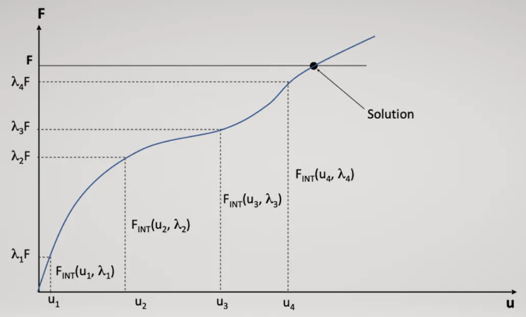
The global equilibrium equation of the nonlinear system is {R(u)} = FINT(u) − {F} = {0}.
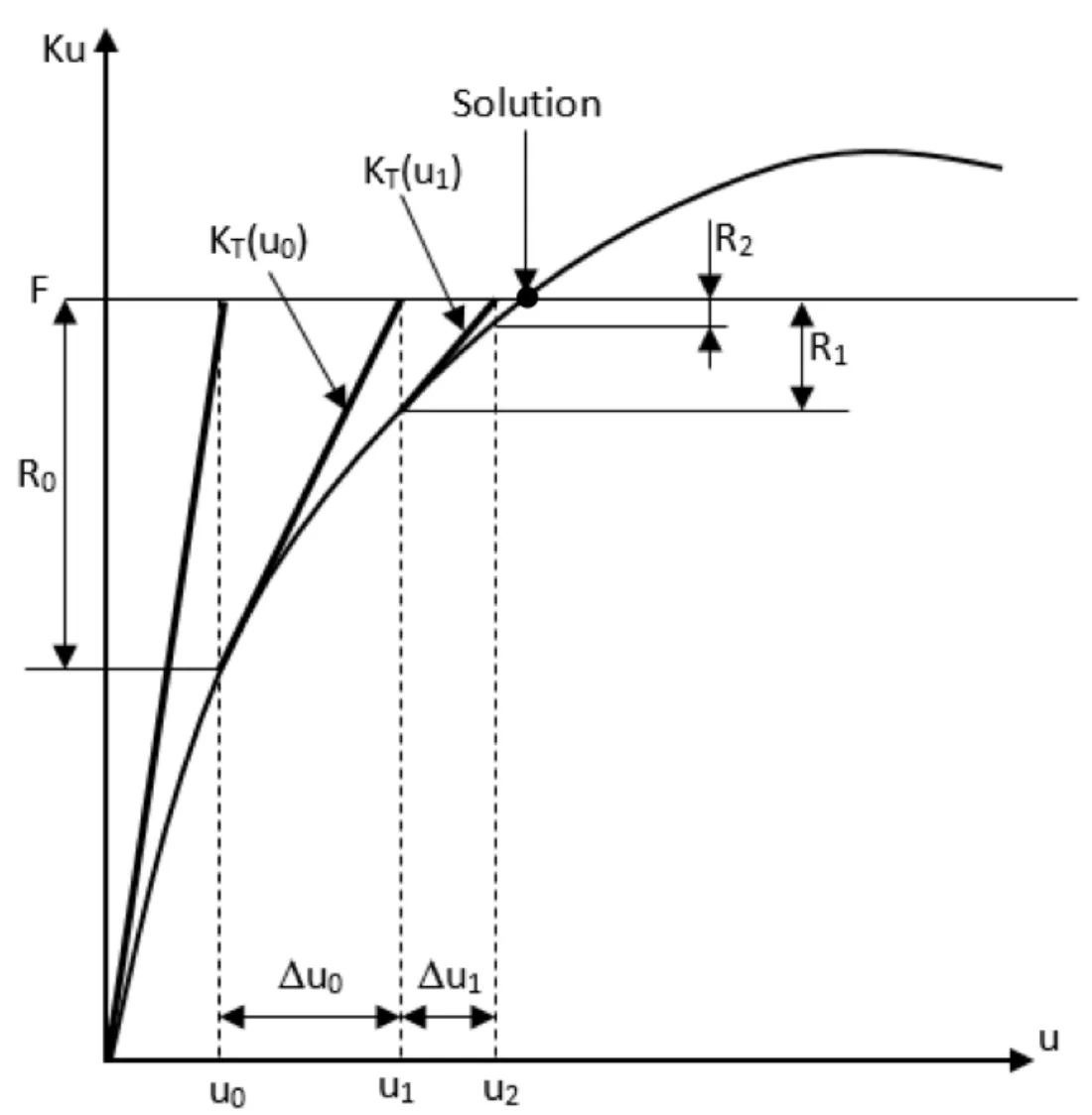
From the first-order Taylor series expansion, the incremental form of the global equilibrium equation is expressed in terms of the incremental nodal displacement {Δu}:

The derivative ∂R/∂u is the Jacobian matrix, also called the tangent stiffness matrix KTi:

The full Newton-Raphson method
- At each iteration, the corresponding tangent stiffness matrix is used to compute the solution.
- The tangent stiffness matrix must be evaluated at each iteration, which is computationally demanding for large problems.
The modified Newton-Raphson method
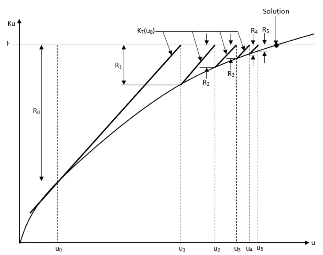
- To improve the performance and reliability of the iterative process, the Newton-Raphson method is slightly modified.
- The tangent stiffness matrix at each iteration is replaced by the stiffness at the initial guess. The tangent stiffness matrix is computed only at the first iteration, and all the following iterations use this initial stiffness matrix.
- More iterations are required, but each iteration is fast, so the computational effort is significantly reduced and the iterative scheme is more stable.
Keep in mind that:
- Loading history is important in nonlinear analysis.
- The Newton-Raphson method converges faster if the initial guess is close to the solution, but you have no control over it.
- Convergence difficulties occur when the applied load is large.
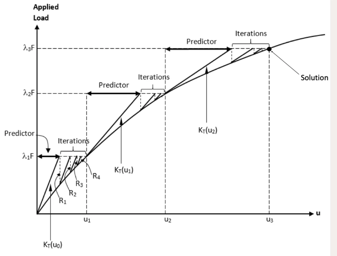
Newton-Raphson combined with the incremental force method
The load is applied in increments. At each increment, a predictor step is followed by Newton-Raphson iterations until equilibrium is reached, and the converged state becomes the starting point of the next increment.
Stiffness matrix update strategies
- When the stiffness of the modeled structure changes significantly, the Newton-Raphson method can diverge unless the tangent stiffness matrix is reevaluated at the critical point.
- You might think that the best approach is to update the stiffness matrix at each iteration.
- However, efficient nonlinear solvers update the stiffness matrix only if the solution may diverge.

Stiffness matrix update processes
- Automatic: the solver selects the most efficient strategy based on convergence rates. At each load increment, the number of iterations required to converge is estimated, and the stiffness matrix is updated if this estimate exceeds a number defined by the user, or if the solution diverges.
- Semi-automatic: for each load increment, the solver performs a single iteration based on the new load, updates the stiffness matrix, and then resumes the solution in automatic mode.
- Iteration-based: the solver updates the stiffness matrix after a number of iterations specified by the analyst, and at convergence.
Convergence criteria
A convergence criterion measures how well the obtained solution satisfies equilibrium. Three criteria are commonly available: residual load, work (energy) and displacement.
The traditional convergence criterion is the residual load, which checks the equilibrium between internal and external forces. The energy-based criterion, which uses both displacements and loads, is also recommended.
Balance accuracy and economical solutions:
- A loose tolerance leads to inaccurate results.
- Too tight a tolerance means too much effort is spent obtaining unnecessary accuracy.
Recommended values: model without contact
| Model type and desired accuracy | Residual load tolerance | Work tolerance |
|---|---|---|
| Very high | 10−3 | 10−3 |
| High | 10−2 | 10−3 |
| Engineering | 10−2 | 10−2 |
| Preliminary design | 10−1 | 10−1 |
Recommended values: model with contact
| Model type and desired accuracy | Residual load tolerance | Work tolerance |
|---|---|---|
| Very high | 10−3 | 10−3 |
| Engineering | 10−3 | 10−3 |
Choosing the incremental load step
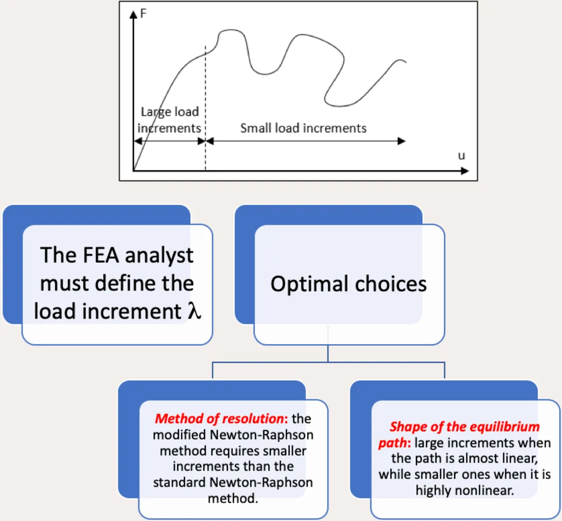
The FEA analyst must define the load increment λ. The optimal choice depends on:
- The method of resolution: the modified Newton-Raphson method requires smaller increments than the standard Newton-Raphson method.
- The shape of the equilibrium path: use large increments where the path is almost linear, and smaller ones where it is highly nonlinear.
How to select the right iterative solution scheme
The choice of the solution scheme depends on the degree of nonlinearity.
| Full Newton-Raphson (standard method) | Modified Newton-Raphson | |
|---|---|---|
| Stiffness matrix update | At each iteration of each load step | Only at the first iteration of each load step |
| Load vector update | At each iteration of each load step | At each iteration of each load step |
| Computational cost | High | Medium to low |
| Solution accuracy | High | Medium |
| Nonlinearity category | Strong: rapid changes in material properties, significant changes in geometric configuration | Medium to moderate: smooth material properties, small changes in geometric configuration |
Strategies to avoid and solve convergence issues
Non-convergence may be due to:
A rigid body motion, caused by bad boundary conditions or a contact support that does not engage. It generally produces very large or infinite displacements. Fix: redefine the boundary conditions (single-point constraints and/or contacts).
Too large a residual, meaning a large difference between the external and internal loads (imbalance of the structure). Fix: reduce the load increments, or change the iterative solution scheme.
Continue with part 3: convergence problems and common mistakes.
Go further
This Book Byte is taken from Chapter 21 of Practical Finite Element Analysis for Mechanical Engineers by Dominique Madier. The topic is covered in depth, with worked examples, in the on-demand course Practical Nonlinear FEA.
See the Practical Nonlinear FEA course Take the free FEA diagnostic