Nonlinear static analysis, part 1: what makes a system nonlinear

Real structures do not always respond in proportion to the loads applied to them. This first part of the nonlinear static analysis series explains what a nonlinear system is, the three types of nonlinearity, and the characteristics that make a nonlinear analysis fundamentally different from a linear one.

What is a nonlinear system?

• A nonlinear system is one whose behavior is not equal to the sum of its parts.
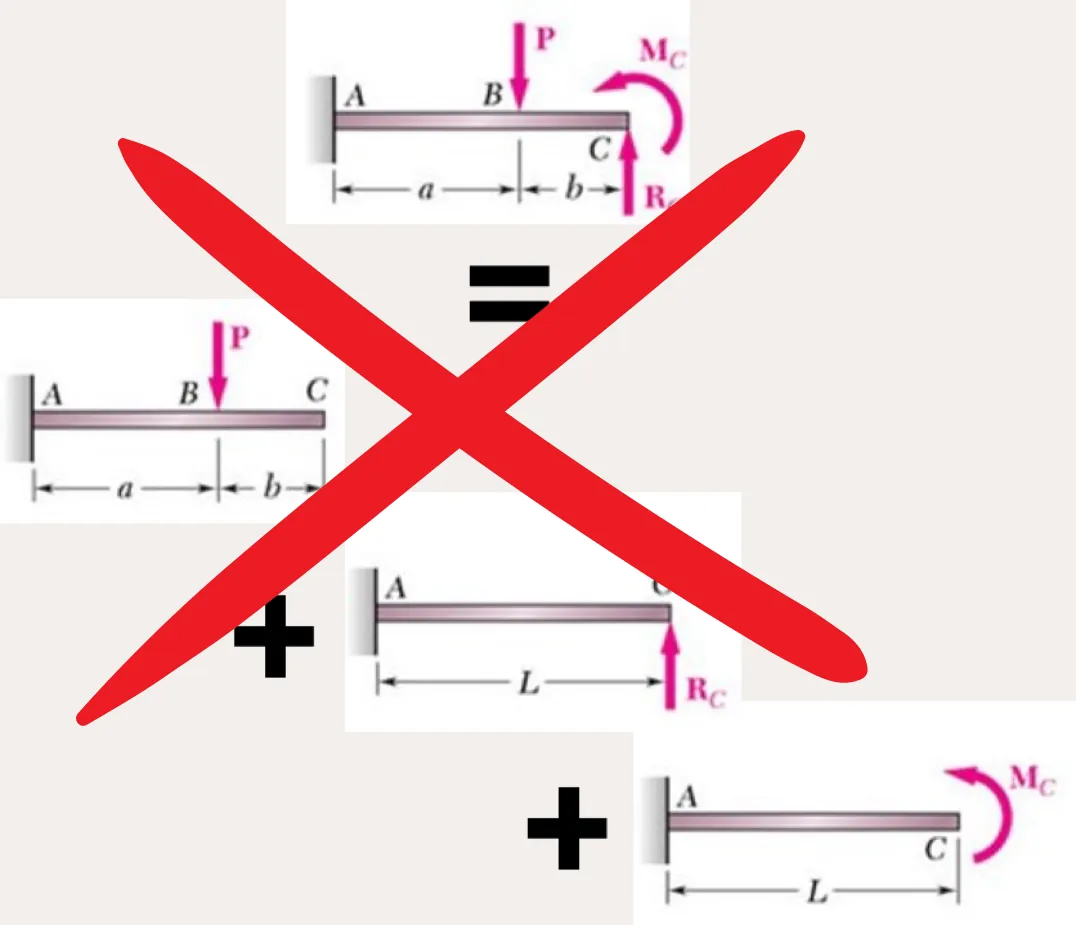
• The behavior of a nonlinear system does not satisfy the principle of superposition.
• In a linear analysis, the response of the structure is assumed to be linearly proportional to the applied loads. In real life, this response may not be proportional.
• In linear static analysis, the stiffness [K] of the analyzed structure is assumed to be constant.
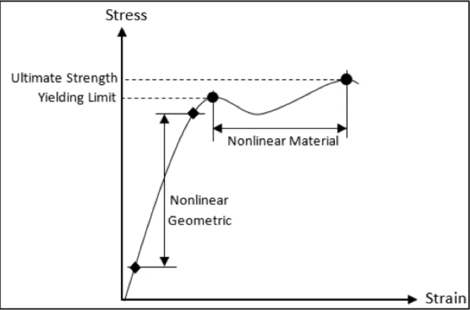
• A structure may behave in a nonlinear manner for geometric, material or boundary reasons.

The stiffness of a structure depends on its geometry and material properties. In a linear analysis, these parameters are assumed to remain unchanged while the loading is applied. In a nonlinear analysis, their changes are taken into account: the stiffness matrix is updated using the deformed configuration of the structure after each load increment.

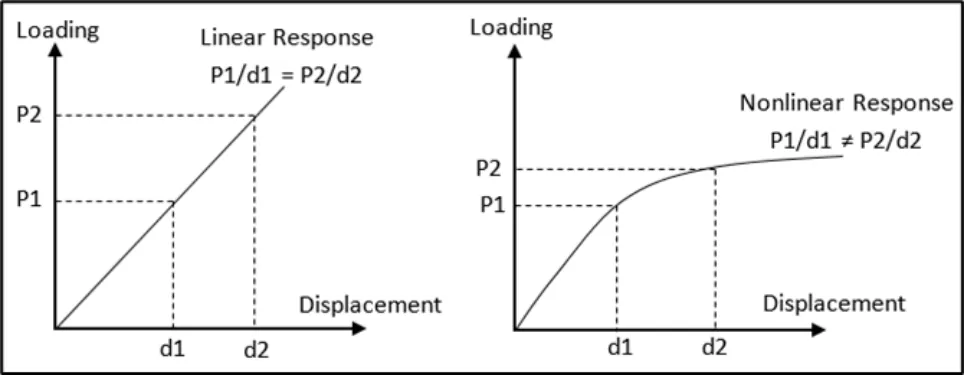
The types of nonlinearity

• Geometric nonlinearity
• Material nonlinearity
• Boundary nonlinearity

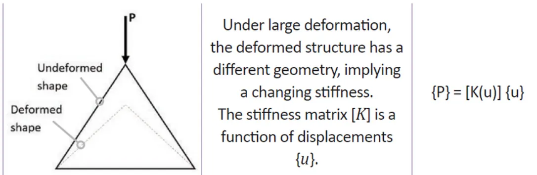
Geometric nonlinearity

• If a body undergoes large deformations, the strain-displacement relations become nonlinear, and the stiffness of the system changes with deformation.
• Under large deformation, the deformed structure has a different geometry, which implies a changing stiffness. The stiffness matrix [K] is a function of the displacements {u}: {P} = [K(u)]{u}.
• Stress stiffening (tension-bending coupling): the bending stiffness of an element increases because of the tension carried by the membrane.

Material nonlinearity

If a material does not follow Hooke's law, nonlinear material models must be used. The stiffness response depends on deformation: the stiffness matrix [K] is a function of the displacements {u}, so {P} = [K(u)]{u}.

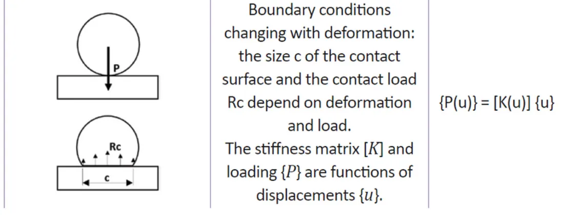
Boundary nonlinearity

The most frequent boundary nonlinearities are found in contact problems. The boundary conditions change with deformation: the size of the contact surface and the contact load depend on the deformation and the load. Both the stiffness matrix [K] and the loading {P} are functions of the displacements {u}: {P(u)} = [K(u)]{u}.

Characteristics of a nonlinear system

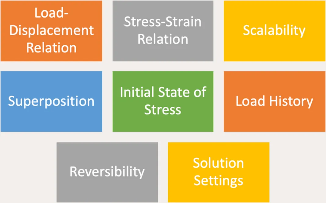
Load-displacement relation

• The stiffness of the analyzed structure is not constant and varies with the applied loads.
• The displacements (translations and rotations) are large and are not related to the original stiffness of the structure.

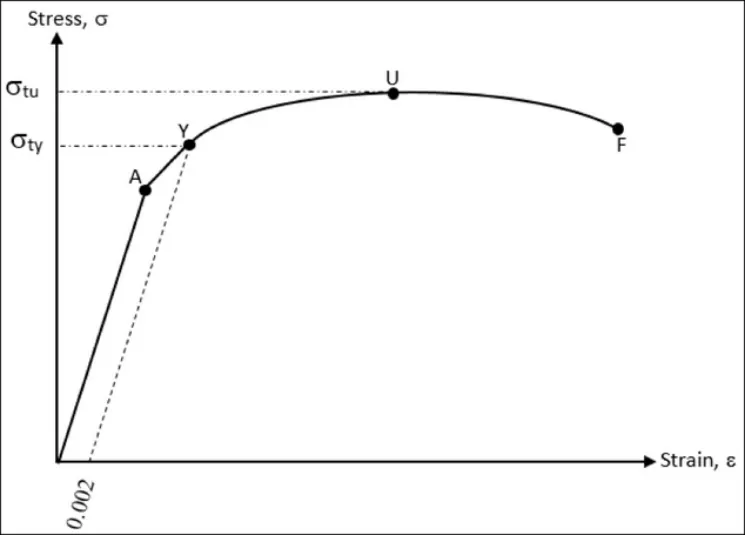
Stress-strain relation

Stresses and strains are not related by a linear function.

Scalability

The results of a nonlinear analysis cannot be scaled: doubling the load does not double the response.

Superposition

The principle of superposition cannot be applied: the response to a combination of loads is not the sum of the responses to each load.

Initial state of stress

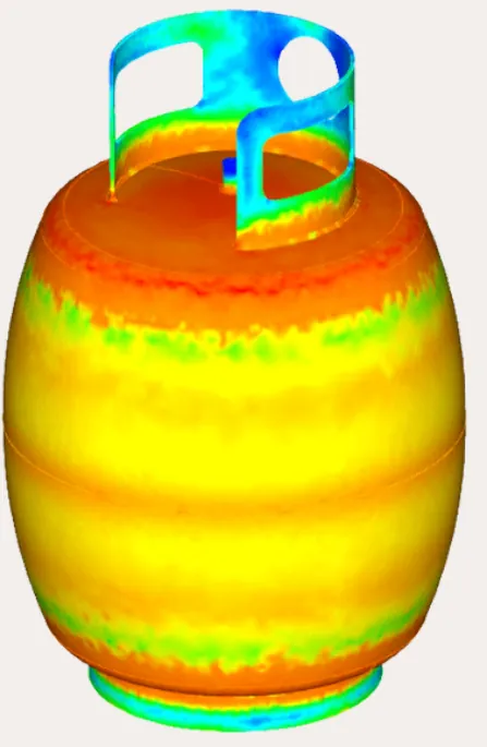
• The initial state of stress (residual stresses, temperature, pre-stressing) may be extremely important in the overall response.
• Only a nonlinear solution can take this initial state into account.

Load history

• The structure's response depends on the load history: it is influenced by the loading sequence.
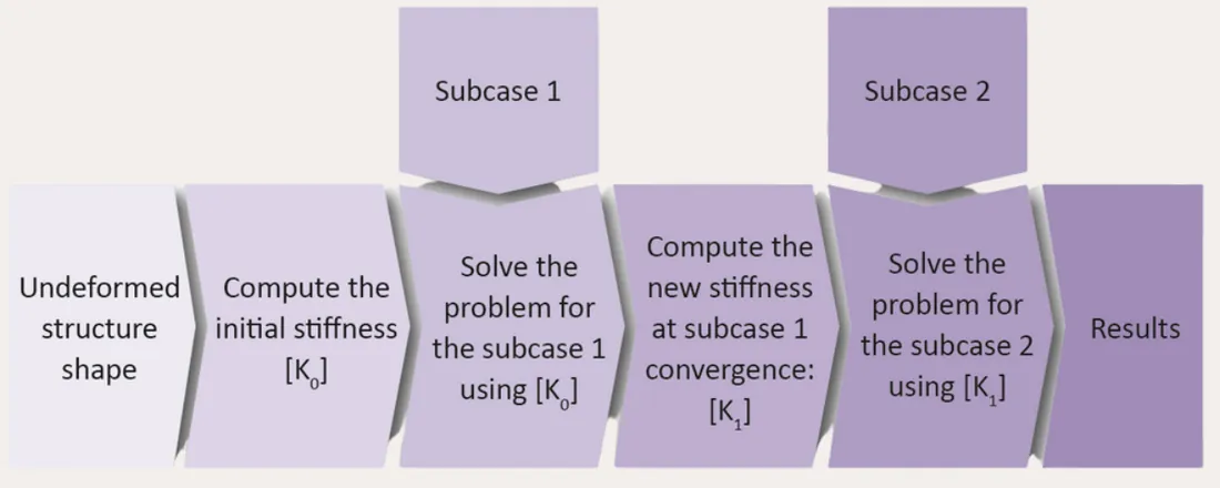
• When several subcases are applied in sequence, the end of one subcase is the initial condition of the next:
  • Undeformed structure shape
  • Compute the initial stiffness [K₀]
  • Solve subcase 1 using [K₀]
  • Compute the new stiffness at the convergence of subcase 1, [K₁]
  • Solve subcase 2 using [K₁]
  • Results

Reversibility

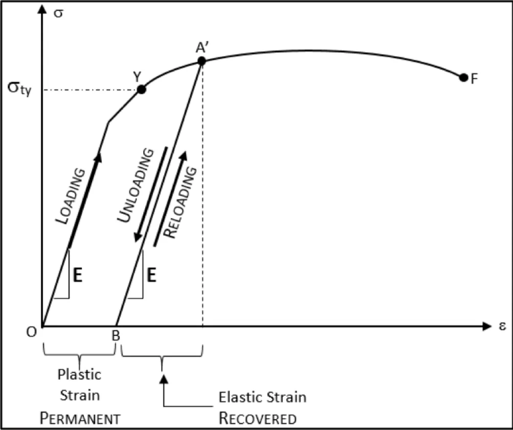
The deformation of the structure is not fully reversible once the applied loads are removed: after yielding, unloading leaves a permanent plastic strain, and only the elastic strain is recovered.

Solution settings

• The external loads are applied in small increments.
• Iterations are performed to ensure that equilibrium is satisfied at each load increment.
• The user must monitor the solution to ensure convergence.
• The computing time is usually large.
• Nonlinear problems may not converge, and may even produce an incorrect solution at convergence.

Continue with part 2: how FEA solvers compute nonlinear problems.

See all Book Bytes