Linear static analysis: assumptions, solution steps and characteristics

What is linear static analysis?

The definition of linear static analysis lies in two words:

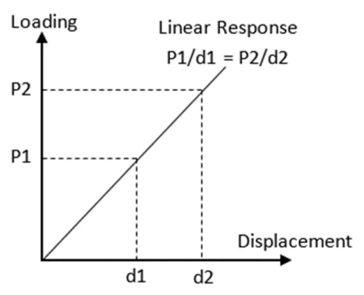
• Linear: the relationship between the external effect applied to the system and the response of the system is linear.
• Static: the external effect applied to the system does not depend on time.

The assumptions of a linear static analysis

When you choose to run a linear static solution, you implicitly make the following assumptions:

1. The deformations are small.
2. The loading and boundary conditions do not change in magnitude or direction during the analysis.
3. The material properties are elastic.
4. The relationship between loads and displacements follows Hooke's law (F = Kx).
5. The results are independent of load history.

How to solve a linear static problem

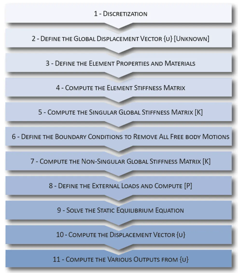
To solve a problem with linear static analysis, the following basic steps are followed:

1. Discretization
2. Define the global displacement vector {u} (unknown)
3. Define the element properties and materials
4. Compute the element stiffness matrices
5. Compute the singular global stiffness matrix [K]
6. Define the boundary conditions to remove all free body motions
7. Compute the non-singular global stiffness matrix [K]
8. Define the external loads and compute {P}
9. Solve the static equilibrium equation
10. Compute the displacement vector {u}
11. Compute the various outputs from {u}

Discretization

The analyzed structure is divided into small, discrete elements connected at nodes (also called grid points). This step is also called meshing.

The stiffness matrix is computed

• The FEA analyst selects the element types compatible with the behavior to be captured.
• The stiffness matrix of each element is computed in matrix form.
• The global stiffness matrix is assembled.
• The global stiffness matrix is singular, meaning that the structure can move as a free body without producing any internal forces in its components.

The boundary conditions and loading are defined

• Constrain the model in all directions; otherwise, the stiffness matrix remains singular, and the solver finds no solution.
• Applying adequate boundary conditions gives a reduced, non-singular global stiffness matrix, representing the constrained structure.
• The analyst provides the loading data. All the external loads applied to the model are combined to form the load vector {P}.

The static equilibrium equation is solved

The linear static equilibrium matrix equation {P} = [K]{u} is solved, where:

• {u} is the vector of the displacements at the nodes of the discretized structure, the unknown of the equation
• [K] is the global stiffness matrix of the structure
• {P} is the applied load vector

LDL^T decomposition methods (Gaussian elimination) are used to solve the system and find {u}.

Various outputs are computed

Once the displacements at the nodes are known, outputs such as element forces, strains and stresses are computed for each element.

The six characteristics of a linear static analysis

1. Load-displacement relationship: K is constant. The changes in geometry due to displacement are small, the undeformed shape of the structure is the reference state, and the displacements vary linearly with the applied loads.
2. Stress-strain relationship: the strains and stresses in the structure are directly proportional through the Young's modulus. There is no elastic limit.
3. Scalability: if an applied load P produces a displacement d, then a load 2P causes a displacement 2d.
4. Superposition: load cases can be combined. If a load P1 produces a displacement d1 and a load P2 a displacement d2, then the load P1 + P2 causes a displacement d1 + d2.
5. Reversibility and load history: the structure's response does not depend on load history, and the structure is assumed to be fully reversible once the applied loads are removed.
6. Solution settings: the external loads are applied in one step, no user interaction with the solver is required during the solution, and the computing time is usually small.

See all Book Bytes