
You do not need to be a mathematician to use FEA well, but you do need to understand what the solver does with your model. This Book Byte explains the equilibrium equation behind every structural FEA, how element stiffness matrices are assembled into the global stiffness matrix, what degrees of freedom are, and how the solver obtains the displacements.
From a continuous system to a discrete system
A real structure, such as an aircraft, is a continuous system subjected to continuous phenomena. Structural idealization turns it into a discrete system: the finite element model.

For continuum mechanics problems, the unknown quantities of the mathematical model are the nodal displacements. The finite element method is based on the following matrix equation, which defines the state of equilibrium of the forces acting on the structure:
[M]{ü} + [B]{u̇} + [K]{u} = P(t)
| Term | Meaning |
|---|---|
| [M] | Mass matrix |
| [B] | Damping matrix |
| [K] | Stiffness matrix |
| {ü} | Acceleration vector |
| {u̇} | Velocity vector |
| {u} | Displacement vector |
| P(t) | Applied load (excitation) |
Variations of the equilibrium equation for different structural problems
The variations of the general equilibrium equation are used to solve different types of structural problems:
- Static analysis: [K]{u} = P
- Buckling analysis: ([K] + λ[Kd]){φ} = λP
- Vibration analysis: ([K] − λ[M]){φ} = 0
- Transient and frequency response analysis: [M]{ü} + [B]{u̇} + [K]{u} = P(t)
where λ is the i-th eigenvalue, {φ} the i-th eigenvector and [Kd] the differential stiffness matrix (also called geometric stiffness).
Assembly of the stiffness matrix from local to global coordinates
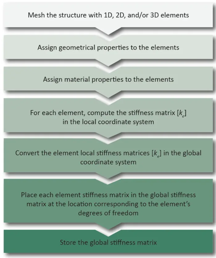
The process is shared between the analyst and the FEA solver.
The analyst's tasks:
- Mesh the structure with 1D, 2D and/or 3D elements.
- Assign geometrical properties to the elements.
- Assign material properties to the elements.
The FEA solver's tasks:
- For each element, compute the stiffness matrix [ke] in the local coordinate system.
- Convert the element local stiffness matrices [ke] to the global coordinate system.
- Place each element stiffness matrix in the global stiffness matrix at the location corresponding to the element's degrees of freedom.
- Store the global stiffness matrix.
Element stiffness matrix
For each element of the structural mesh, the stiffness matrix is computed in the element local axis system and transformed to a global coordinate system common to all elements.
The characteristics of the stiffness matrix are:
- The stiffness matrix is square.
- The stiffness matrix is symmetric.
- All diagonal terms are positive.
Global stiffness matrix
The element stiffness matrices are assembled into a unique global stiffness matrix, depending on how the elements are connected.
The stiffness at a node is obtained by summing the stiffness of all the elements connected to that node.
Assembling the global stiffness matrix of a structure consists of placing each degree of freedom of each element in its proper position in the global stiffness matrix of the whole structure.
Degrees of freedom
In FEA, the degrees of freedom (DOF) are the fundamental variables. In solid mechanics and structural analysis, the degrees of freedom are the translations and rotations at the nodes of the discretization. Not all types of DOF are necessarily transmitted by all types of elements.

The DOF concept is fundamental to understanding:
- how loads can be applied
- how boundary conditions restrain the model
- how the different types of elements can be connected
A translational DOF means that a force can be transmitted through a node, while a rotational DOF means that a moment can be transmitted through a node.
How the FEM equations are solved
With the direct method, the equilibrium equation {P} = [K]{u} is solved for the unknown displacements {u} without inverting [K].
An efficient and accurate method is the LDLT decomposition. This method can be viewed as the matrix form of Gaussian elimination.
The three steps of the LDLᵀ method
- Factorization: [K] = [L][D][L]T, using the Cholesky decomposition.
- Forward substitution: {P} = [K]{u} = [L]{y}, solved for {y}.
- Backward substitution: {y} = [D][L]T{u}, solved for {u}.


Go further
This Book Byte is taken from Chapter 5 of Practical Finite Element Analysis for Mechanical Engineers by Dominique Madier. The topic is covered in depth, with worked examples, in the on-demand course Practical Basic FEA.
See the Practical Basic FEA course Take the free FEA diagnostic