
Linear buckling analysis gives a fast estimate of stability, but it can be dangerously optimistic for real structures. This Book Byte explains when a nonlinear buckling analysis is needed, what it lets you predict, how to read the load history path to distinguish real buckling from numerical instability, how to analyze post-buckling, and the essential steps of any nonlinear analysis.
Why perform a nonlinear buckling analysis?
Linear buckling analysis (LBA) assumes small displacements and stresses below the yield point.
- If the structure exhibits large displacements and the stresses exceed the proportional limit, a nonlinear buckling solution is necessary to predict structural instability.
- LBA can be dangerous, because it produces overestimated buckling factors for complex problems.
- LBA cannot estimate the behavior after buckling, and it does not take nonlinear behaviors into account.

Nonlinear buckling analysis allows you to:
- Consider the influence of buckling on structural stiffness
- Evaluate the stress distribution in the structure once buckling occurs
- Determine the structure's post-buckling response
As in a nonlinear static analysis, the applied loading is gradually increased to determine the first limit point, which is the maximum load before the solution becomes unstable.
The following features can be included in a nonlinear buckling analysis:
- Large deformations (geometric nonlinearity)
- Plastic behavior (material nonlinearity)
- Contacts
- Any combination of the above
What a nonlinear buckling analysis gives you
The outcomes of a nonlinear buckling analysis are much richer than those of LBA:
- Actual deformations: while LBA only provides a shape, without real displacements, nonlinear buckling shows the actual deformations of the structure and their values before and after failure.
- History path: presented as a graph, it shows how your structure behaves, since you have access to the state of equilibrium of the structure at each load increment.
- Failure animation: you can observe the collapse of the structure and its sequence.
- Post-buckling response: you obtain not only the response up to instability, but also how the structure responds after instability occurs.
The history path and the converged analysis
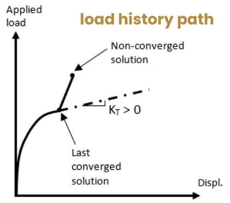
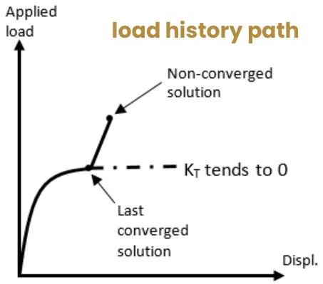
The buckling load can be found by reviewing the load history path (the deflection versus load curve). Output enough result steps to be able to examine the load history path.
A non-converged solution does not necessarily mean that the structure has reached its maximum capacity. The risk is confusing physical instability (real buckling) with numerical instability (false buckling).
To detect real buckling, investigate the tangent stiffness:
- It is close to zero near real buckling.
- A nearly flat load history path indicates physical instability.
Post-buckling
In a nonlinear buckling analysis, you can examine what happens in a structure after buckling: this is called post-buckling analysis. When the structure has reached its critical limit, you may want to know whether it can still carry load.
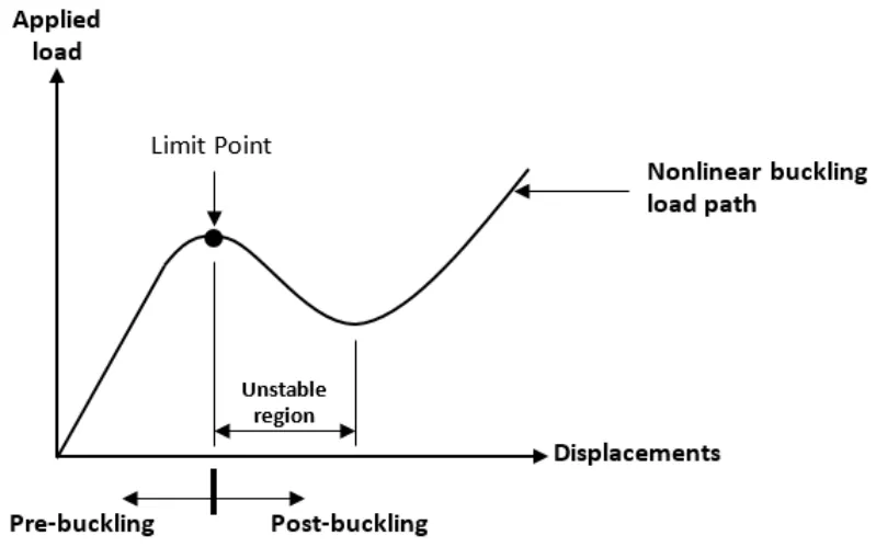
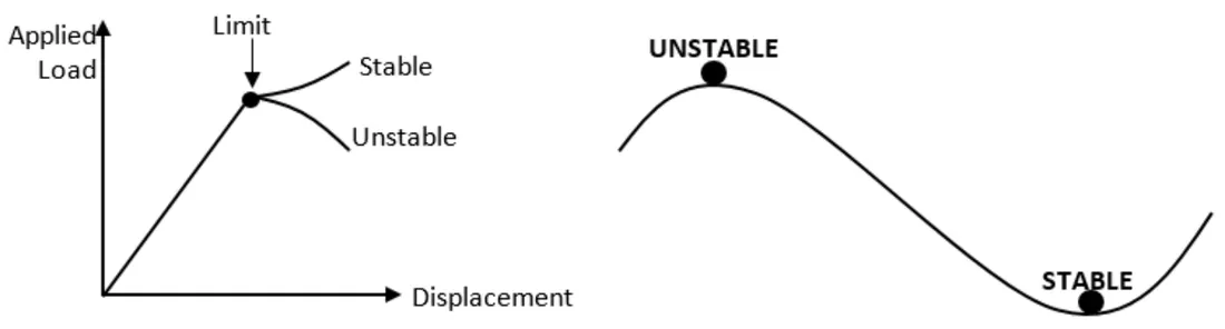
Mathematically speaking, buckling is a bifurcation problem: when a limit point is reached, there is more than one solution. Two paths are possible from the limit point, and the secondary path can be of two types:
- Stable post-buckling: the structure continues to carry the applied load while maintaining stiffness (positive definite stiffness matrix). This is the least dangerous situation. However, if you miss it during the iterative process, you will underestimate the stresses and the load-carrying capacity of the structure.
- Unstable post-buckling: the structure loses its stiffness and can no longer carry the same load. It exhibits very large geometrical changes.
The Newton-Raphson method is not always the appropriate solution scheme for post-buckling. It only works if the post-buckling path is stable, which is difficult to know in advance. Therefore, arc-length methods (Crisfield and Riks methods) are recommended for post-buckling analyses, because they work for both stable and unstable post-buckling paths.

Essential steps in nonlinear analysis
Step 1: understand your problem and the structural behavior. Finite element analysis requires a thorough understanding of the structural behavior of the phenomenon you wish to simulate. Produce a simplified model using linear static and linear buckling analyses: it will reveal which regions of your model will experience nonlinear responses, and at which load levels.
Step 2: precisely define your goal and the objective of your analysis. You must know the precise questions you want your analysis to answer, and set up your model accordingly. All your assumptions are conditioned by the objective of the analysis.
Step 3: understand your FEA software. FEA software has specificities in its solution settings and in how it outputs results and warnings. It is good to know how the software reports divergence or bad boundary conditions. Take the time to read the software documentation, and prepare a simple model to make sure you understand all the details.
Step 4: verify and validate the results of the nonlinear solution.
- Verification: is the model computed correctly from a numerical point of view?
- Validation: has the correct model been computed?
Go further
This Book Byte is taken from Chapter 23 of Practical Finite Element Analysis for Mechanical Engineers by Dominique Madier. The topic is covered in depth, with worked examples, in the on-demand course Practical Nonlinear FEA.
See the Practical Nonlinear FEA course Take the free FEA diagnostic